Conditional Quantile Regressions
Because no-one is average
Introduction
Question: What are quantiles? and why do we care??
Quantiles provide a better characterization of distributions.
- It provides you with more information than standard summary statistics (means and variance)
How so? In general, there are 3 ways you can use to know “everything” about a distribution.
You either have access to every single \(y_i\)
Or you know the distribution function \(f(y)\) (pdf)
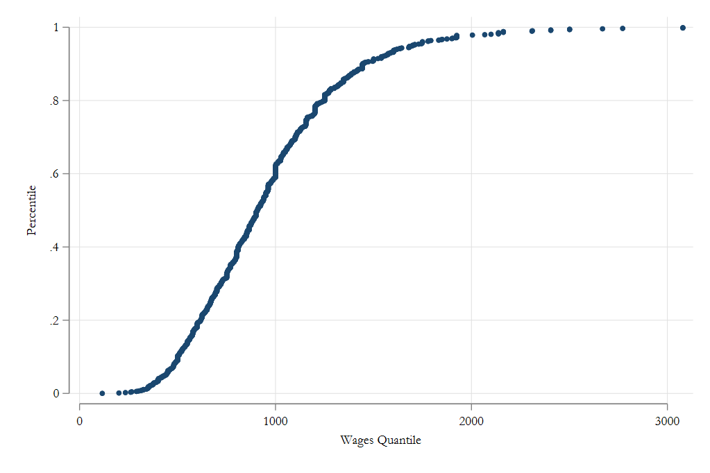
Or you know the cumulative distribution function \(F(y)=\int_\infty^y f(t) dt = P(Y\leq y)\)
However, there is an additional way. Quantile:
\[ Q(\theta) = F^{-1}(p) \]
\(Q(\theta) = F^{-1}(\theta)\)
Other advantages? Yes!
Quantiles are far more stable in the presence of outliers. Because of this, they are particularly useful as measures of central tendency (perhaps superior to the mean) (🤔?)
- Simple “test”. In the small town of Troy-NY one of the residents wins the 2B$ lottery. How much has welfare increase for the average resident?
Scaled IQR can be used as an alternative measure of dispersion.
\[ se2 = \frac{Q_{75}-Q_{25}}{1.34898} \]
- They are also “function-transformation” resistant: \(exp(Q_{log(y)} (.10)) = Q_y(.10)\)
- And are also very easy to estimate:
- Sort data by \(y\) \(\rightarrow\) Obtain weighted ranks \(\rightarrow\) choose the lowest value so that \(\theta\) % of the data is less of equal to that number
\[ F^{-1} (tau) = inf(x: F(x)\geq t) \]
- This “just” requires obtaining an approximation for \(F(\theta)\), which can be approximated using nonparametric methods!
\[\hat F(x) = \frac{1}{N}\sum (K_F(x,x_i,h)) = \frac{1}{N}\sum 1(x_i<x) \]
- then we simply “invert” the function for whichever quantile we are interested in.
Technical Note
There are many empirical ways to estimate quantiles, even when using the empirical distribution function.
So do not be suprised about small differences in the estimates.
When using Smooth functions, the choice of the kernel is also important. (and bandwidth)
Statistical Inference
As with the mean, sampling quantiles are measured with sampling error.
However their standard errors are not as intuitive to obtain ( but can be derived using the delta Method)
\[Q_y(\tau) = F_y^{-1}(\tau) \rightarrow F_y(Q_y(\tau)) = \tau \ || \ \frac{\partial}{\partial \tau} \]
This gives us: \[f_y(Q_y(\tau)) \frac{dQ}{d\tau} =1 \rightarrow \frac{dQ}{d\tau} = \frac{1}{f(Q_y(\tau))} \]
So we have:
\[ \begin{aligned} \hat Q_y(\tau) &\simeq Q_y(\tau) + \frac{1}{f(Q_y(\tau))}(\hat \tau-\tau) \\ \hat Q_y(\tau) - Q_y(\tau) &\simeq \frac{1}{f(Q_y(\tau)}(\hat \tau-\tau) \\ Var(\hat Q_y(\tau)) &= \frac{Var(\hat \tau - \tau) }{f^2(Q_y(\tau))} = \frac{N^{-1} \tau(1-\tau)}{f^2(Q_y(\tau))} \end{aligned} \]
Lets understand this elements
Quantile SE
\[ Var(\hat Q_y(\tau)) = \frac{Var(\hat \tau - \tau) }{f^2(Q_y(\tau))} = \frac{1}{f^2(Q_y(\tau))}\frac{\tau(1-\tau)}{N} \]
The variance of a quantile depends on the distribution of \(\tau\). This follows a Bernoulli distribution: Is \(y\geq Q_y\) or \(y<Q_y\).
- Largest near the center of the distribution (50%-50%) but smaller (more precise) near the tails of the distribution.
But also depends on the density of the distribution.
- More precise estimates when the density is high (center), but less precise near tails of the distribution.
- And, because \(f()\) is unknown, there is another source of variation.
And as usual, it depends on the sample size (N)
Of course, you also have the alternative method. Bootstrap!
Example
Using Bootstrap
frause wage2, clear
bootstrap q10=r(r1) q25=r(r2) q50=r(r3) ///
          q75=r(r4) q90=r(r5), reps(1000) nodots: ///
          _pctile wage  , p(10 25 50 75 90)
warning: _pctile does not set e(sample), so no observations will be excluded
         from the resampling because of missing values or other reasons. To
         exclude observations, press Break, save the data, drop any
         observations that are to be excluded, and rerun bootstrap.

Bootstrap results                                        Number of obs =   935
                                                         Replications  = 1,000

      Command: _pctile wage, p(10 25 50 75 90)
          q10: r(r1)
          q25: r(r2)
          q50: r(r3)
          q75: r(r4)
          q90: r(r5)

------------------------------------------------------------------------------
             |   Observed   Bootstrap                         Normal-based
             | coefficient  std. err.      z    P>|z|     [95% conf. interval]
-------------+----------------------------------------------------------------
         q10 |        500   9.149192    54.65   0.000     482.0679    517.9321
         q25 |        668   14.21654    46.99   0.000     640.1361    695.8639
         q50 |        905   15.19745    59.55   0.000     875.2135    934.7865
         q75 |       1160   20.87954    55.56   0.000     1119.077    1200.923
         q90 |       1444   32.84186    43.97   0.000     1379.631    1508.369
------------------------------------------------------------------------------
Analytical SE
sort wage
gen w1 = _n
gen w0 = _n-1
by wage:gen p=0.5*(w1[_N]+w0[1])/935
kdensity wage, at(wage) gen(fwage) nodraw
gen se = sqrt(p*(1-p)/935)/fwage
tabstat wage se if inlist(wage,500,668,905,1160,1444), by(wage)
Summary statistics: Mean
Group variable: wage (monthly earnings)

    wage |      wage        se
---------+--------------------
     500 |       500  13.27634
     668 |       668  14.78419
     905 |       905  14.69217
    1160 |      1160   19.3574
    1444 |      1444  29.32711
---------+--------------------
   Total |  730.7619  15.88035
------------------------------
From \(Q_Y\) to \(Q_{Y|X}\)
The approaches used earlier to identify a particular quantile are not the only ones.
Just like we can use OLS to estimate Means, we could also use a similar method to estimate the median.
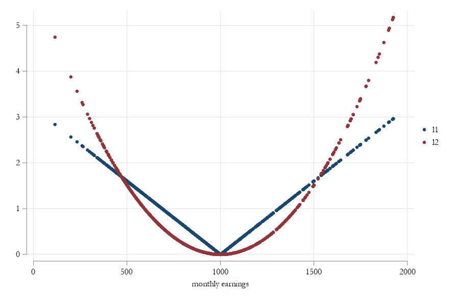
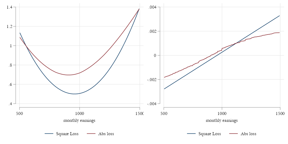
We only need to change the loss function \(L()\) from an \(L^2\) to a \(|L|\).
Consider this:
\[\begin{aligned} median(Y) &= min_\mu \frac{1}{N}\sum |y-\mu| \\ &=\frac{2}{N}\sum (y-u)(0.5-I([y-u]<0) \end{aligned} \]
Q and Loss functions
- The loss function for Quantiles does not penalize “errors” as much as \(L^2\) does.
- This is why its more robust to outliers (almost not affected by them).
- However, the loss function is no longer differentiable (is discontinuous). So requires other methods to find the solution. Even if it may not look like that:
From \(\beta\) to \(X\beta\)
Koenker and Bassett (1978) extended this approximation in two ways:
Allowing for Covariates (\(X's\)) variation
Allowing to identify other quantiles in the distribution:
\[ \beta(\tau) = \underset {b}{min} \ N^{-1} \sum \rho_\tau(y_i-X_i'b) \\ \rho_\tau (u) = u (\tau-I(u<0)) \]
- This implicitly states that you want to find a combination of \(X's\) such that \(\tau\) proportion of \(y_i\) are lower than the \(X_i'\beta(\tau)\), for every combination of \(X's\).
- Or as close as possible.
Interpretation: Why is it so different from OLS?
- In Rios-Avila and Maroto(2022) we stress that OLS can be interpreted at different “levels”. Consider the following:
\[ y_i = b_0 + b_1 x_1 + b_2 x_2 + e \]
If the errors are exogenous, and there is no heteroskedasticty, you can “obtain” marginal effects at many levels
\[ Ind: \frac{dy_i}{dx_{1i}}=b_1 \]
If \(x_1i\) changes, and everything else is fixed, then \(y_i\) changes by \(b_1\) units for that individual.
\[\begin{aligned} E(y_i|X=x)&=b_0 + b_1 x_1 + b_2 x_2 \\ \frac{dE(y|x)}{dx_1} &=b_1 \\ \end{aligned} \]
If \(x_1\) changes for a group of individuals with the same characterisitcs, everything else is fixed, then everyone in that group will experience a change in \(Y\) by \(b_1\) units.
\[\begin{aligned} E(y_i) &= b_0 + b_1 E(x_1) + b_2 E(x_2) \\ \frac{dE(y)}{dE(x_1)} &=b_1 \end{aligned} \]
If \(E(x_1)\) changes for everyone, then the overall average change in \(Y\) is \(b_1\) units.
- So in OLS, assuming a linear model in parameters, Nothing changes. The effect is the same! (although magnitude of the “experiment” changes)
But CQreg?
For quantile regressions, things are not that simple.
There is no “individual” level quantile effect, because we do not observe individual ranks \(\tau\).
- If we could observe them, and we assume they are fixed, then one can obtain individual level effects.
Because \(\tau\) is unobserved, all Qregression coefficients, should be interpreted as effects on Conditional Distributions (thus the name CQREG).
- In other words, effects are just expected changes in some points in the distribution.
You cannot use it for unconditional effects either (not easily), because
\[ E(Q_{Y|X}(\tau)) \neq Q_Y(\tau) \]
and you cannot “simply” average the CQREG effects to get unconditional quantiles.
what does it mean?
This means that CQREG interpretation are percentile \(\tau\) and covariate \(X\) specific.
Fixed rank. If you happen to be on the top of the distribution (and stay there), the quantile effect is given by the \(\beta(\tau)\)
Rank is not fixed: What we see is the effect of a change in \(X\) on the conditional distribution of \(Y\) (measured by the quantile)
So this must be kept in mind, whenever one interpret results
Visualizing Differences in Interpretation
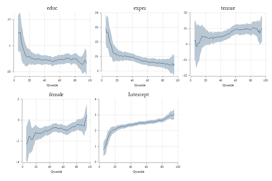
Example: Wages…
frause oaxaca, clear
qui:qreg  lnwage educ exper tenure female, nolog q(10)
est sto m1
qui:qreg  lnwage educ exper tenure female, nolog q(50)
est sto m2
qui:qreg  lnwage educ exper tenure female, nolog q(90)
est sto m3
* ssc install estout
esttab m1 m2 m3, se nogaps mtitle(q10 q50 q90)
(Excerpt from the Swiss Labor Market Survey 1998)
------------------------------------------------------------
(1) (2) (3)
q10 q50 q90
------------------------------------------------------------
educ 0.103*** 0.0694*** 0.0639***
(0.0166) (0.00433) (0.00902)
exper 0.0200*** 0.00758*** 0.00402
(0.00493) (0.00128) (0.00267)
tenure 0.000669 0.00657*** 0.00774*
(0.00603) (0.00157) (0.00327)
female -0.151 -0.0689** -0.0543
(0.0806) (0.0210) (0.0437)
_cons 1.462*** 2.474*** 2.984***
(0.219) (0.0570) (0.119)
------------------------------------------------------------
N 1434 1434 1434
------------------------------------------------------------
Standard errors in parentheses
* p<0.05, ** p<0.01, *** p<0.001Example: Wages…
qregplot educ exper tenure female, cons q(5/95)
Other Interpretations of Qreg
Random coefficents
One approach to both understanding, and simulating QREG is by also understanding the intuition behind the data generating process.
\[ \begin{aligned} y &= b_0(\tau)+b_1(\tau)x_1 + +b_2(\tau)x_2+...+b_k(\tau) x_k \\ \tau &\sim runiform(0,1) \end{aligned} \]
where all coefficients are a function (preferably monotonically increasing or decreasing) of \(\tau\) .
We want them to be monotonically increasing or decreasing because we want that \[ X \beta(\tau_1 ) \geq X \beta(\tau_2 ) \ \text{ if } \ \tau_1 > \tau_2 \]
In this specification the unobserved component \(\tau\) is similar to luck. If you are lucky and get a high \(\tau\) then you will have better outcomes than anyone of your peers.
Also notice: \(\tau\) is the only random factor, and should be uncorrelated with \(X\) (you do not make your luck!)
SVC model with a latent running variable
Another way of thinking about Qreg is to align it to the semiparametric method we introduced ealier. SVC model.
In SVC, there is an observed running variable \(z\), and we focus on analyzing how the “local” effects of \(X\) on \(Y\) change as a function of \(z\).
The difference with Qreg is that the running variable is unknown \(\tau\).
- Given the outcome, and characteristics we can identify something like a “latent” component.
- There are a few (recent) papers that focus on estimation and identification of these models. The general intuition is that the qreg model is identified by the following moment condition:
\[ E\Big( 1[x\beta(\tau) - y > 0 ] - \tau \Big) = 0 \]
but substitute the indicator function with a smooth function. CDF
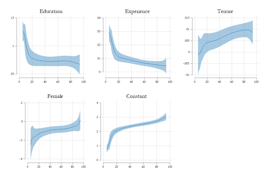
\[ E\Big( F(x\beta(\tau) - y) - \tau \Big) = 0 \]
Being differentiable, this problem is relatively easier to solve (given good initial values)
Example (with sivqr)
Scale and Location Model
Another approach that can be used to understand Quantile regressions (and elaborate the interpretation) is to assume that the coefficients are in fact capturing two components:
\[y = Xb + Xg(\tau) \]
Location: \(Xb\) which indicates what is the average/typical relationship between X and Y.
Scale: \(Xg(\tau)\) which indicates how far one could be from the average effect, given a relative rank \(\tau\)
Estimation of this model is not standard. But can be manually implemented:
- Estimate OLS and get residuals
- Estimate QREG using those residuals
Requires additional care for the estimation of SE
Scale and Location 2: Heteroskedasticity
A second approach that is useful to understand and interpret CQreg is to consider a parametric version of the LS model:
\[y = Xb + \gamma (X) * e \text{ with } \gamma(X)>>0\]
This shows the relationship between a quantile regressions and heteroskedasticity in the error term.
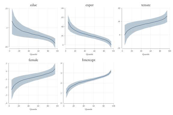
If we assume Heteroskedasticity is parametric (\(\gamma(x) = X \gamma\)), it constrains the relationship across all quantile coefficients:
\[y = X(b+\gamma F^{-1}(\tau)) \rightarrow b(\tau)=b+\gamma\times q(\tau) \]
- Making it more efficient, albeit imposing constrains of the relationship.
Example (with mmqreg)
Estimation and Statistical Inference
As hinted previously, there are many approaches that can be used for the estimation of Conditional Quantile regressions.
Official:
qreg,sqreg,bsqreg,iqregCContributed:
qreg2,qrprocess,mmqreg,smqreg,sivqrFor Standard errors, however, there are main 3 options. Under the assumption of iid error. Non iid error (robust), and assuming clustered standard errors.
\[ \begin{aligned} iid: \Sigma_\beta &=\frac{\tau(1-\tau)}{N f^2_y(F^{-1}(\tau))}(X'X)^{-1} \\ niid: \Sigma_\beta &= \tau(1-\tau) (X'f(0|x)X)^{-1} \ (X'X) \ (X'f(0|x)X)^{-1} \\ alt: \Sigma_\beta &= (IF_\beta \ ' IF_\beta) N^{-2} \end{aligned} \]
Or simply Bootstrap
Problems and Considerations
Unless otherwise specified, quantile regressions are linear in variables (and parameters?)
With few exceptions, quantile regressions are quantile specific. Comparisons across quantiles require joint estimation (to construct VCV matrix)
Because they are “local” estimators, there is risk of crossing quantiles. (Violation of Monotonicity)
Non-linear effects will be present if either the location or scale components are nonlinear.
Quantile regressions are very sensitive to measurement errors in both dependent and independent variables
They can be difficult to interpret (see references)
Implementation of fixed effects is not straightforward
Quantile Regressions with Fixed Effects
The problem
- There are two problems related to Estimating Quantile Regressions with (multiple) Fixed Effects
- First: As with nonlinear models, Adding many fixed effects creates an incidental parameter problem.
- Second: For Conditional Quantile Regressions, it can be difficult to interpret the role of fixed effects.
Simulating some data
clear
set obs 1000
gen id = _n
gen vi = rnormal()
gen ui = rnormal()+vi

gen toexp = 1+rpoisson(5)
expand toexp
gen err = rnormal()
gen x1 = rnormal()+vi+err
gen x2 = rnormal()+vi+err
gen y = 1+x1+x2+ui+rnormal()*exp(0.2*x1-0.2*x2+0.3*ui)
Number of observations (_N) was 0, now 1,000.
(5,019 observations created)Accounting for Fixed effects
Benchmark
Assume you observe those fixed effects:
Code
------------------------------------------------------------
                      (1)             (2)             (3)
                      q10             q50             q90
------------------------------------------------------------
x1                  0.780***        0.988***        1.219***
                 (0.0190)        (0.0139)        (0.0224)
x2                  1.219***        1.000***        0.763***
                 (0.0189)        (0.0138)        (0.0223)
ui                  0.654***        1.000***        1.352***
                 (0.0180)        (0.0132)        (0.0212)
_cons              -0.458***        0.970***        2.420***
                 (0.0236)        (0.0173)        (0.0279)
------------------------------------------------------------
N                    6019            6019            6019
------------------------------------------------------------
Standard errors in parentheses
* p<0.05, ** p<0.01, *** p<0.001
Ignoring Fixed Effects
Code
------------------------------------------------------------------------------------------------------------
                      (1)             (2)             (3)             (4)             (5)             (6)
                      q10             q50             q90             m10             m20             m30
------------------------------------------------------------------------------------------------------------
x1                  0.981***        1.171***        1.470***        0.780***        0.988***        1.219***
                 (0.0235)        (0.0217)        (0.0415)        (0.0190)        (0.0139)        (0.0224)
x2                  1.339***        1.260***        1.139***        1.219***        1.000***        0.763***
                 (0.0234)        (0.0215)        (0.0412)        (0.0189)        (0.0138)        (0.0223)
ui                                                                  0.654***        1.000***        1.352***
                                                                 (0.0180)        (0.0132)        (0.0212)
_cons              -1.133***        0.813***        3.275***       -0.458***        0.970***        2.420***
                 (0.0300)        (0.0276)        (0.0529)        (0.0236)        (0.0173)        (0.0279)
------------------------------------------------------------------------------------------------------------
N                    6019            6019            6019            6019            6019            6019
------------------------------------------------------------------------------------------------------------
Standard errors in parentheses
* p<0.05, ** p<0.01, *** p<0.001
Solution 1: Correlated Random Effects
Idea: Include “PAnel average” of all indep variables as regressors.
They should control (at least partially) for the unobserved effects.
\[Q_p(y|X) = X\beta + \alpha \bar X + \epsilon\]
Code
------------------------------------------------------------------------------------------------------------
                      (1)             (2)             (3)             (4)             (5)             (6)
                      q10             q50             q90             m10             m20             m30
------------------------------------------------------------------------------------------------------------
x1                  0.825***        0.972***        1.195***        0.780***        0.988***        1.219***
                 (0.0250)        (0.0246)        (0.0460)        (0.0190)        (0.0139)        (0.0224)
x2                  1.176***        1.023***        0.774***        1.219***        1.000***        0.763***
                 (0.0252)        (0.0248)        (0.0463)        (0.0189)        (0.0138)        (0.0223)
x1p                 0.310***        0.413***        0.663***
                 (0.0575)        (0.0565)         (0.106)
x2p                 0.283***        0.406***        0.551***
                 (0.0564)        (0.0555)         (0.104)
ui                                                                  0.654***        1.000***        1.352***
                                                                 (0.0180)        (0.0132)        (0.0212)
_cons              -0.951***        0.861***        3.146***       -0.458***        0.970***        2.420***
                 (0.0278)        (0.0273)        (0.0511)        (0.0236)        (0.0173)        (0.0279)
------------------------------------------------------------------------------------------------------------
N                    6019            6019            6019            6019            6019            6019
------------------------------------------------------------------------------------------------------------
Standard errors in parentheses
* p<0.05, ** p<0.01, *** p<0.001
Solution 2: FE are Fixed
- Canay (2011) proposes make the “simplifying” that “Fixed effects” are constant across quantiles.
- Thus a two step procedure is proposed:
- First: Estimate the fixed effects using OLS
- Second: Estimate the quantile regression using outcome after taking FE “off”
\[\begin{aligned} y &= X\beta + \alpha_i + \epsilon \\ Q_\tau(y - \hat \alpha_i |X) &= X\beta(\tau) + \epsilon_\tau \\ \end{aligned} \]
Code
(4 missing values generated)

------------------------------------------------------------------------------------------------------------
                      (1)             (2)             (3)             (4)             (5)             (6)
                      q10             q50             q90             m10             m20             m30
------------------------------------------------------------------------------------------------------------
x1                  0.727***        0.992***        1.277***        0.780***        0.988***        1.219***
                 (0.0213)        (0.0120)        (0.0218)        (0.0190)        (0.0139)        (0.0224)
x2                  1.117***        1.004***        0.853***        1.219***        1.000***        0.763***
                 (0.0212)        (0.0119)        (0.0216)        (0.0189)        (0.0138)        (0.0223)
ui                                                                  0.654***        1.000***        1.352***
                                                                 (0.0180)        (0.0132)        (0.0212)
_cons              -0.296***        1.021***        2.336***       -0.458***        0.970***        2.420***
                 (0.0272)        (0.0153)        (0.0277)        (0.0236)        (0.0173)        (0.0279)
------------------------------------------------------------------------------------------------------------
N                    6015            6015            6015            6019            6019            6019
------------------------------------------------------------------------------------------------------------
Standard errors in parentheses
* p<0.05, ** p<0.01, *** p<0.001
Solution 3: Modified Canay(2011)
- Same as before, but rather than “removing” fixed effects, we control for them in the model:
\[\begin{aligned} y &= X\beta + \alpha_i + \epsilon \\ Q_\tau(y |X) &= X\beta(\tau) + \gamma \hat \alpha_i + \epsilon_\tau \\ \end{aligned} \]
Code
------------------------------------------------------------------------------------------------------------
                      (1)             (2)             (3)             (4)             (5)             (6)
                      q10             q50             q90             m10             m20             m30
------------------------------------------------------------------------------------------------------------
x1                  0.800***        0.993***        1.171***        0.780***        0.988***        1.219***
                 (0.0182)        (0.0137)        (0.0206)        (0.0190)        (0.0139)        (0.0224)
x2                  1.193***        1.006***        0.831***        1.219***        1.000***        0.763***
                 (0.0181)        (0.0137)        (0.0205)        (0.0189)        (0.0138)        (0.0223)
fe                  0.691***        0.991***        1.279***
                 (0.0159)        (0.0120)        (0.0180)
ui                                                                  0.654***        1.000***        1.352***
                                                                 (0.0180)        (0.0132)        (0.0212)
_cons              -0.334***        1.017***        2.354***       -0.458***        0.970***        2.420***
                 (0.0227)        (0.0171)        (0.0257)        (0.0236)        (0.0173)        (0.0279)
------------------------------------------------------------------------------------------------------------
N                    6015            6015            6015            6019            6019            6019
------------------------------------------------------------------------------------------------------------
Standard errors in parentheses
* p<0.05, ** p<0.01, *** p<0.001
Solution 4: LS model
- Machado and Silva (2019) propose a different approach. They suggest modeling the quantile regression using linear models for a scale and location model.
- This simplifies the task of estimating multiple equations:
\[\begin{aligned} y &= X\beta + \epsilon \\ \hat\epsilon^2 &= X\gamma + \nu \\ Q\left( \frac{\hat\epsilon}{X\gamma}\right) &= q(\tau) \\ \beta(\tau) &= \beta + \gamma \times q(\tau) \end {aligned} \]
qui:mmqreg y x1 x2   , q(10)  abs(id) robust
est sto m1
qui:mmqreg y x1 x2   , q(50)  abs(id) robust
est sto m2
qui:mmqreg y x1 x2 , q(90) abs(id) robust
est sto m3
esttab m1 m2 m3 m10 m20 m30, se nogaps mtitle(q10 q50 q90)
------------------------------------------------------------------------------------------------------------
                      (1)             (2)             (3)             (4)             (5)             (6)
                      q10             q50             q90             m10             m20             m30
------------------------------------------------------------------------------------------------------------
main
x1                  0.780***        0.993***        1.214***        0.780***        0.988***        1.219***
                 (0.0183)        (0.0147)        (0.0203)        (0.0190)        (0.0139)        (0.0224)
x2                  1.231***        0.992***        0.745***        1.219***        1.000***        0.763***
                 (0.0197)        (0.0162)        (0.0233)        (0.0189)        (0.0138)        (0.0223)
ui                                                                  0.654***        1.000***        1.352***
                                                                 (0.0180)        (0.0132)        (0.0212)
_cons              -0.346***        1.017***        2.431***       -0.458***        0.970***        2.420***
                 (0.0220)        (0.0207)        (0.0251)        (0.0236)        (0.0173)        (0.0279)
------------------------------------------------------------------------------------------------------------
N                    6019            6019            6019            6019            6019            6019
------------------------------------------------------------------------------------------------------------
Standard errors in parentheses
* p<0.05, ** p<0.01, *** p<0.001
Next topic…Unconditional Quantiles
Unconditional Quantile Regressions and RIF-Regressions
