Diff in Diff: From 2x2 to GxT DID

Advances, Problems and Solutions

Fernando Rios-Avila

Levy Economics Institute of Bard College

Why differences in diffences?

• Differences-in-Differences (DID) is one of the most popular tools in applied economics for analyzing causal effects of an intervention or policy treatment.

• Under reasonable assumptions, DID allows you to identify these effects by comparing changes in the treatment group with changes in the control group.

  • This method of identification even allows for controlling for self-selection in the treatment.

• In recent years, several advances in DID have been developed, revealing issues with the traditional DID design, particularly with the application of TWFE.

• Today, I will briefly present the problems and solutions that have been proposed, and how they are implemented in Stata.

• So lets Start with the basics: 2x2 DID

2x2 DID: Cannonic Design

• In the 2x2 DID design, we have 2 groups:
  • Control (\(D=1\)) y treated (\(D=0\)),
• Which are observed for two periods of time:
  • Before (\(T=0\)) and after (\(T=1\)) the treatment.
• For all groups and periods of time, we observe the realized outcome \(Y\), but cannot observe all potential outcomes.
• This setup is valid both for panel data and repeat cross-sections, but will focus on panel data.

Potential outcomes and Treatment Effects

• Potential outcomes are the outcomes we would observe for each observation in the data if it were assigned to either the treatement or control group.

  • \(Y_{i,t}(D=0)\): Potential outcome for individual \(i\) at time \(t\) if he was never treated.
  • \(Y_{j,s}(D=1)\): Potential outcome for individual \(j\) at time \(s\) if he was treated.

• However, we are only able to observe one of this outcomes: \[Y_{i,t} = Y_{i,t}(1)D_i + Y_{i,t}(0)(1-D_i)\]

• Where \(D_i\) is a dummy indicates the effective treatment status of individual \(i\).

• Now, we are interested in Treatment Effects for \(i\), or any summary measures, after the treatment is applied:

\[TE = Y_{i,1}(1)-Y_{i,1}(0) \text{ or } ATT =E(Y_{i,1}(1)-Y_{i,1}(0)|D=1)\]

The DID Estimator: Assumptions

• Because we can’t observe both potential outcomes, we need to make assumptions to identify the treatment effect.

1. Stable Unit Treatment Value Assumption (SUTVA): The treatment status of one unit does not affect the potential outcomes of other units. (No spillovers)

2. Parallel Trends: In the absence of treatment, in average, both groups would have followed the same trend (changes) over time.

\[\color{blue}{E(Y_{i,1}(0) - Y_{i,0}(0)|D_i=1)} = \color{green}{E(Y_{i,1}(0)-Y_{i,0}(0)|D_i=0)}\]

3. No Anticipation: Before the treatment takes place (\(T=0\)), the potential outcomes do not depend on the treatment status.

\[Y_{i,0}(0) = Y_{i,0}(1)\]

The DID Estimator

• Lets take a second look at the ATT definition: \[\begin{aligned} ATT &=E(Y_{i,1}(1)|D=1)-\color{red}{E(Y_{i,1}(0)|D=1)} \\ &=E(Y_{i,1}|D=1)-\color{red}{E(Y_{i,1}(0)|D=1)} \end{aligned} \]

• The problem is to estimate the red component, to obtain an estimator for the ATT.

• However, under the PTA and No Anticipation, the observed part can be written as: \[E(Y_{i,1}(0)|D=1) = E(Y_{i,1}-Y_{i,0}|D=0) + E(Y_{i,0}|D=1) \]

• Which gives the usual ATT estimator:

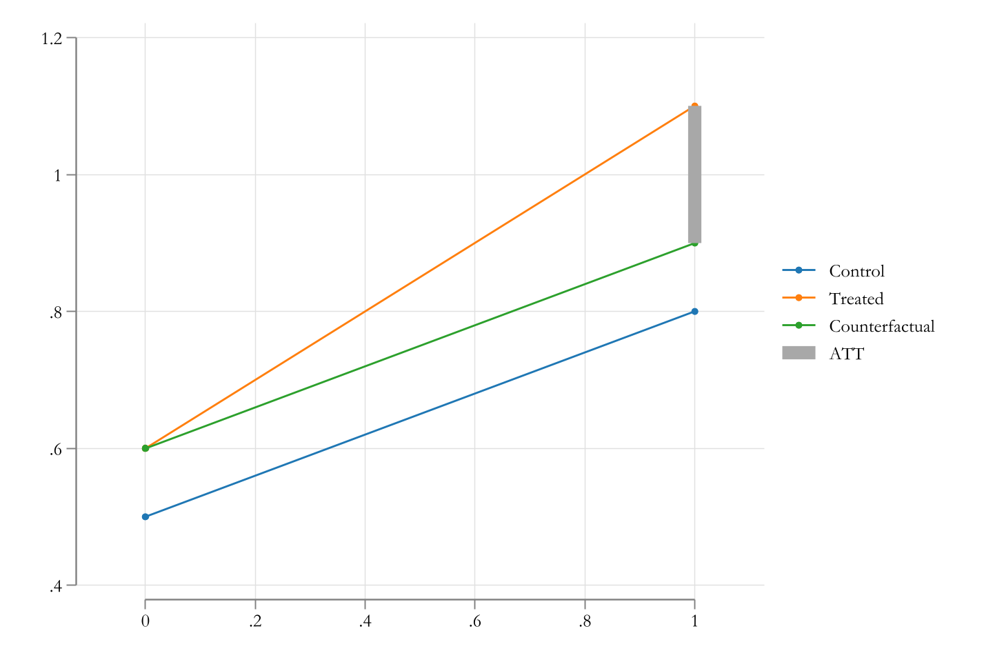
\[ATT =\underbrace{E(Y_{i,1} - Y_{i,0}|D=1)}_{\Delta treat} - \underbrace{E(Y_{i,1}-Y_{i,0}|D=0)}_{\Delta control}\]

Graphically

checking did_imputation consistency and verifying not already installed...
installing into c:\ado\plus\...
installation complete.

How to estimate it?

• Difference-in-Means:

\[\widehat{ATT}=\bar Y^{D=1,T=1} - \bar Y^{D=1,T=0} - [ \bar Y^{D=0,T=1} - \bar Y^{D=0,T=0} ]\]

• Regression:

\[Y_{i,t} = \beta_0 + \beta_1 D_i + \beta_2 t + \beta_3 (D_i \times t) + \epsilon_{i,t}\]

• With Panel Data: Fixed Effects

\[\begin{aligned} Y_{i,t} &= \beta_0 + \sum \delta_i + \beta_2 t + \beta_3 (D_i \times t) + \epsilon_{i,t} \\ \Delta Y_{i} &= \beta_2 + \beta_3 D_i + \epsilon_{i} \text{ for } t=0 \\ \end{aligned} \]

Extension: Adding Controls

• The DID estimator presented above relies on Unconditional Parallel Trends. It may work if both control and treated groups are similar in all aspects, except for the treatment. But they may not.
• In this case, we can add controls to the model, to account for differences in the groups.

\[Y_{i,t} = \beta_0 + \beta_1 D_i + \beta_2 t + \beta_3 (D_i \times t) + X_{it} \gamma + \epsilon_{i,t}\]

• But this would be wrong. Why?

Problems of Adding Controls

• Simply adding controls imposes assumption of homogenous treatement effects. As described in Sant’Anna and Zhao (2020), \(\gamma\) may not be the same as the ATT.
  • Solution: Interactions between controls and all group\time dummies: \[y_{i,t} = \beta_0 + \sum \delta_i + \beta_2 t + \beta_3 (D_i \times t) + X_{it} \gamma + \sum \gamma_x (X-\bar X_{D\times T})*D*T + \epsilon_{i,t}\]
• Controlling for time varying variables may introduce biases (bad controls)
  • Solution: use only pre-treatment variables as controls. (panel) or variables that should not be affected by the treatment (cross-sections)
  • Also: If using Panel Data, one can add as controls all variables history. (see for example Caetano and Callaway (2022))

Potential Solution: Sant’Anna and Zhao (2020)

• DID is a straighforward estimator, that relies strongly on the Unconditional Parallel Trends Assumption. (UPTA)

• One solution to the problem is to use the Conditional Parallel Trends Assumption (CPTA), which can be less restrictive.

• This states that PTA holds, only after conditioning on a set of variables \(X\). (looking at subgroups).

\[\color{blue}{E(Y_{i,1}(0) - Y_{i,0}(0)|D_i=1,X)} = \color{green}{E(Y_{i,1}(0)-Y_{i,0}(0)|D_i=0,X)}\]

• So, if you can “control” for individual characteristics, you could estimate the treatment effect, and still report Average Treatment Effects for the population.

\[ATT = E\big[ [E(Y_{i,1}(0) - Y_{i,0}(0)|D_i=1,X ] \big]\]

Added Assumption

• When accouting for covariates, one needs to add an additional assumption to the data:

• There is an overlap in the distribution of \(X\) between the treated and control groups. (common support)

\[0 << Pr(D=1|X) << 1\]

• This is important, because if there is no overlap, the treatment effect cannot be identified for all groups, and may create distorted estimates.

Potential Solution: drdid, teffects

• Sant’Anna and Zhao (2020) propose various alternatives to estimate the treatment effect with controls, under CPTA. They contrast the implementation of methods that use linear regressions, Inverse Probability Weighting (IPW) and Doubly Robust Estimators (DR).
• Similar estimates could be obtained using teffects in Stata.
• But how does this work? Two Cases:
  • Panel Data: This simplifies the problem, because we can use the Data structure to estimate the model.
  • Crossection: This is more complicated because requires careful consideration of idenfication assumptions, and groups of interest.

Panel Data

• Step 1: Estimate the changes in the outcome \(\Delta Y_i = Y_{i,1} - Y_{i,0}\). (the First D)
  • Because of this, we are implicitly reducing our sample size: from \(N\) to \(N/2\) (because of the unestimated fixed effects)
• Step 2: Estimate the treatment effect:
  • Simplest case, no controls: \[\Delta Y_i = \beta_0 + \beta_1 D_i + \varepsilon_i\]
• In other words, the model is now a simple linear regression, with 1 period.

Panel Data: Adding controls

• Because you have now only 1 period, and two groups. All treatment effect estimators can be used.
  • regression outcome, IPW, doubly robust, matching, etc.
  • We use them to estimate the second D of DID
• Empirically: With Transformed data (\(\Delta y\)) as dependent variable, any of the methods in teffects can be used to estimate the treatment effect.
• With untransformed data (RC), you can use drdid to estimate the treatment effect, and their Standard errors.
  • You need to make sure you have only 2 periods of data.

Panel Data: Methods

• Regression: reg (drdid) or ra (teffects)
  • using \(\Delta y\) as dependent variable, estimate a linear model with covariates (No FE) for the untreated, and predict outcomes. This would become your “Potential outcome change under no-treatment”

\[ ATT = E(\Delta Y_{i}|D=1) - E({\hat\gamma X|D=1})\]

• Inverse Probability Weighting: stdipw (drdid) or ipw (teffects)
  • Estimate the likelihood of being treated, and use it to identify a propensity score and IPW weights \(p(D=1|X) = \hat p(X)\)

\[ ATT = E(\Delta Y_{i}|D=1) - E\left({\Delta Y_{i} \frac{p(X)}{1-p(X)}|D=0}\right)\]

Panel Data: Methods

• Doubly Robust Estimation: dript and dripw (drdid) or ipwra aipw (teffects)
  • Estimate the likelihood of being treated, and use it to identify a propensity score and IPW weights \(p(D=1|X) = \hat p(X)\)
  • Estimate a weighted regression with \(\Delta y\) as dependent variable or estimate a weighted regression correction. (see here slide 17-18) for more details.
  • Combinations of modeling outcome and modeling likelihood and pscores makes the estimator doubly robust.
• For Repeated crossection, the math becomes more complicated to follow and identify the “group of interest”
  
• See here slide 53-54 for more details.

Example

Some Data Preparation

qui:frause lalonde, clear
keep  if treated==0 | sample==2
bysort id (year):gen dy = re[2]-re[1]

(5,574 observations deleted)

Using teffects:

teffects ra (dy educ black married nodegree hisp re74) (experimental) if year==1975 , atet

Iteration 0:  EE criterion =  4.433e-21  
Iteration 1:  EE criterion =  8.994e-26  

Treatment-effects estimation                    Number of obs     =     16,417
Estimator      : regression adjustment
Outcome model  : linear
Treatment model: none
------------------------------------------------------------------------------
             |               Robust
          dy | Coefficient  std. err.      z    P>|z|     [95% conf. interval]
-------------+----------------------------------------------------------------
ATET         |
experimental |
   (1 vs 0)  |  -1055.483   346.1459    -3.05   0.002    -1733.917   -377.0497
-------------+----------------------------------------------------------------
POmean       |
experimental |
          0  |   3118.849   185.0719    16.85   0.000     2756.114    3481.583
------------------------------------------------------------------------------

Using drdid:

drdid re educ black married nodegree hisp re74 , ivar(id) time(year) tr(experimental) reg

Doubly robust difference-in-differences                 Number of obs = 32,834
Outcome model  : regression adjustment
Treatment model: none
------------------------------------------------------------------------------
             | Coefficient  Std. err.      z    P>|z|     [95% conf. interval]
-------------+----------------------------------------------------------------
ATET         |
experimental |
   (1 vs 0)  |  -1055.483   346.1451    -3.05   0.002    -1733.915   -377.0511
------------------------------------------------------------------------------

by hand:

qui:reg dy educ black married nodegree hisp re74 if exper==0
predict dy_hat, xb
gen att_i = dy-dy_hat
tabstat att_i, by(exper) 

Summary for variables: att_i
Group variable: experimental 

experimental |      Mean
-------------+----------
           0 | -9.61e-06
           1 | -1055.483
-------------+----------
       Total | -27.32414
------------------------

Highlights I: Identification

• The identification relies on the non-anticipation assumption and the parallel trends assumption.
  • Neither of these assumptions can be tested, but they can be supported by the data.
• For Implementation, If one has panel data, teffects and drdid can be used to estimate the treatment effect, and their standard errors. (after preparing the data)
• Otherwise, drdid can be used for repeated crossection as well. (or GMM)

Highlighs II: Overlapping

• The overlapping assumption is important, and has different implications for the different methods.
• When the estimation method is reg or ra, the overlapping assumption is less biding, because the model is extrapolates to created “potential outcomes” for the treated group.
  • However, extrapolation may not be accurate, or create incorrect extrapolations (base category dummies)
• With doubly robust methods, the overlapping assumption is more relevant. dript is particularly sensitive to this assumption, and may not even converge if there is weak overlap.
• For most practical purposes, dripw may be the most stable, and preferred method.

Highlighs III: Controls

• With panel data, drdid automatically constrains model specification to use pre-treatment information only.
  • Added work is required to include post-treatment information.
• With Repeated crossection, drdid would use both pre-treatment and post-treatment information.

From 2x2 to GxT DID

How GxT DID was suppoused to work

• While the 2x2 DID design is simple to understand, it does not reflect the type of information that is available in most cases. (G>2 and T>2)

• Until few years ago, when this kind of data was available, the standard approach was to use a generalized DID design, which extended the use of Fixed Effects:

\[ \begin{aligned} 2\times2: Y_{i,t} &= \beta_0 + \beta_1 T + \beta_2 D_i + \beta_3 (D_i \times T) + \epsilon_{i,t} \\ G\times T: Y_{i,t} &= \sum \gamma_t + \sum \delta_i + \theta^{fe} PT_{i,t} + \epsilon_{i,t} \\ \end{aligned} \]

where \(PT_{i,t}\) assume the value of 1 for the treated group After the treatment is applied, and 0 otherwise, and \(\theta^{fe}\) representing the treatment effect.

• Little that we know that this approach only works if the treatment effect is homogeneous across all groups and periods.

Why it doesn’t work?

There are at least two-ways that have been used to explain why the Standard TWFE does not work:

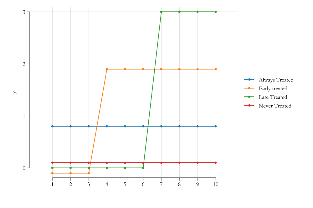
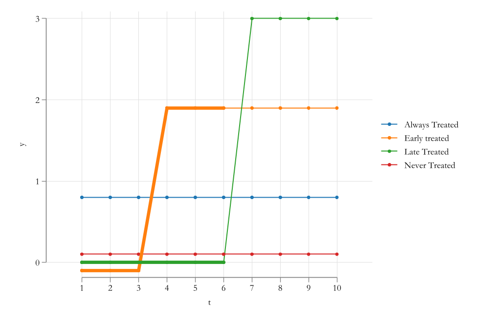
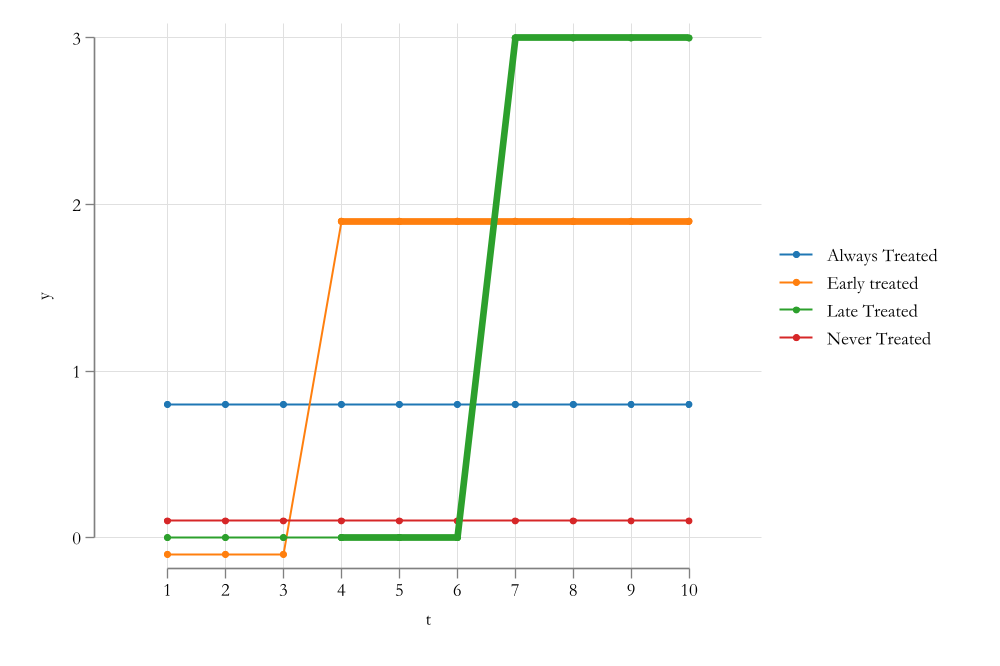
• The “Bad Controls” Problem: Goodman-Bacon (2021) shows that the TWFE estimator for ATT is a kind of weighted average of all possible DID one could estimate. Some of these would not be good DID designs.

• Negative Weights: Chaisemartin and D’Haultfœuille (2020) and Borusyak, Jaravel, and Spiess (2023) show that because TWFE ATT estimator is a weighted average of all group-Specific ATT, some may include negative weights.

  This may produce negative ATT even if all group-specific ATT are positive.

• However, when the treatment effect is homogeneous, Neither of these situations would be a problem.

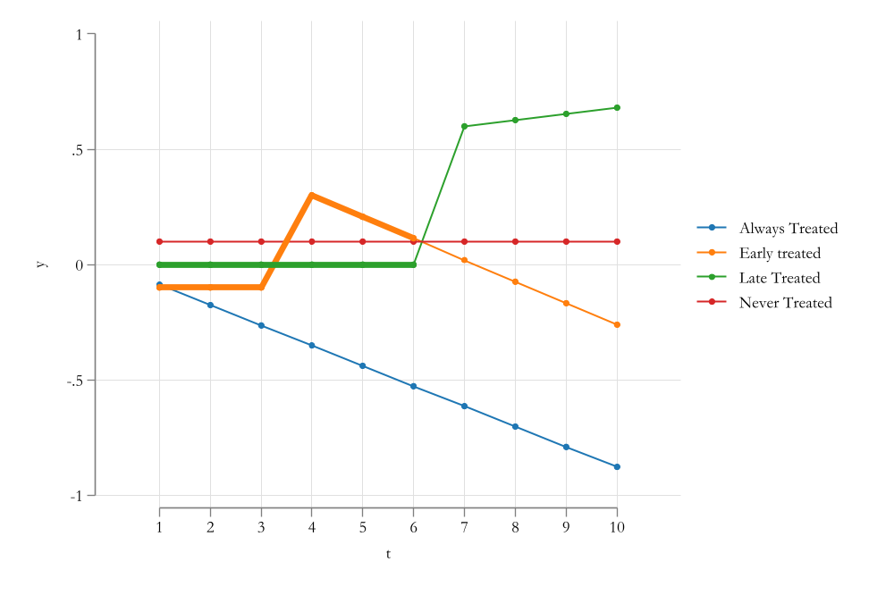
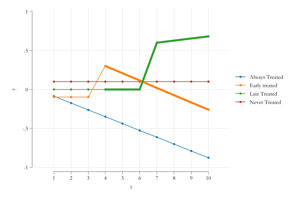
The “Bad Controls” Problem

• All Cases
• Early Treated vs Later Treated (Good)
• Early Treated vs Later Treated (bad)

The “Bad Controls” Problem

• All Cases
• Early Treated vs Later Treated (Good)
• Early Treated vs Later Treated (bad)

Negative Weights

• To understand the idea of Negative Weights, lets consider the following example:

\[Y_{i,t} = \sum \delta_i + \sum \gamma_t + \theta PT + \epsilon_{i,t}\]

If the panel data is balanced, and we apply FWL, we can use partialling out the Fixed Effects:

\[\widetilde{PT}_{it}=PT_{it}-\overline{PT}_{i}-\overline{PT}_{t}+\overline{PT}\]

and estimate \(\theta^{fe}\) as:

\[\hat\theta^{fe} = \frac{\sum \widetilde{PT_{it}} Y_{it}}{\sum \widetilde{PT}_{it}^2} = w_{it} Y_{it} \]

\[\widetilde{PT}_{it}=PT_{it}-\overline{PT}_{i}-\overline{PT}_{t}+\overline{PT}\]

• \(\overline{PT}_{i}\) is the share of periods a unit is observed to be treated. (larger for early treated)
• \(\overline{PT}_{t}\) is the share of units treated at time \(t\). (increasing)
• \(\overline{PT}\) Share of treated “unit-periods”

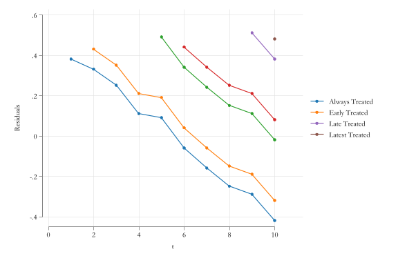
Thus,

• Units that are treated early, (high \(\overline{PT}_{i}\))
• but are analyzed at later periods (\(\overline{PT}_{t}\) increasing in \(t\))

Will be more likely to have a negative weight \(w_{it}\), thus contaminating the ATT estimate.

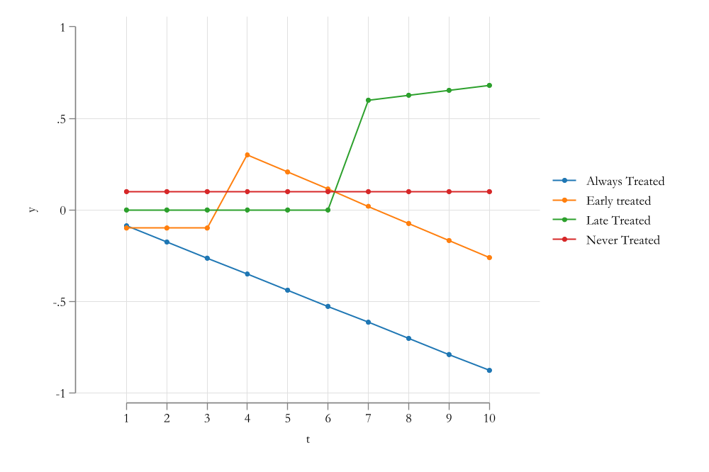
Graphically

Summarizing the Problem

• Both Negative Weights and Bad Controls are capturing the same problem.

1. By using already treated units as controls (bad controls), we are implicitly applying negative weights to units that are already treated.

2. This would not be a problem on its own, if the treatment effect is homogeneous across all groups and periods.

3. However, if the treatment effect is heterogeneous, Parallel Trends between already treated and late treated units may not hold.

GxT DID: Generalized DID

Setup

• In the Generalized DID
  • One has access to multiple periods of data: \(t = 1,2,...,T\).
  • And units can be treated at any point before, during or after the available Data \(G = -k,..1,2,..,T+l\).
    • This is the cohort or group.
  • We also assume that once a unit is treated, it remains treated. (no reversals/no cohort-change)
• From our perspective, units treated at or before \(t=1\) will be considered as Allways treated.
  • This units cannot be used for analysis.
• For any practical purpose, if we do not observe a unit being treated in the window of time observed, we assume its Never Treated.
  • For Notation we say these units belong to \(g=\infty\) (or that they could be treated at some point in the far future)

GxT DID: Generalized DID

Potential Outcomes

• In contrast with previous setup, with the GDID, we believe observations have multiple potential outcomes, for each period of time.
  • \(Y_{i,t}(G)\) is the potenital outcome for individual \(i\) at time \(t\), if this unit would be treated at time \(G\).
  • Thus we state that depending on “when” a unit is treated, the potential outcomes could be different.
  • This is what it means allowing for heterogeneity.

GxT DID: Generalized DID

Parallel Trends Assumption

• PTA assumption is also slightly modified. Because we can differentiate between never-treated and not-yet-treated, one could impose those PTA assumptions.

  Never Treated \[E(Y_{i,t}(\infty) - Y_{i,t-s}(\infty)|G=g) = E(Y_{i,t}(\infty) - Y_{i,t-s}(\infty)|G=\infty) \forall s>0 \]

  Not Yet Treated

  \[E(Y_{i,t}(\infty) - Y_{i,t-s}(\infty)|G=g) = E(Y_{i,t}(\infty) - Y_{i,t-s}(\infty)|G=g') \forall s>0 \]

• Which suggests PTA hold for all pre- and post-treatment periods.

• Some methods only rely on Post-treatment PTA.

GxT DID: Generalized DID

No Anticipation

• As before, we also require no anticipation.
  • That the before treatment takes place (or is announced), the potential outcomes do not depend on the treatment status.

\[Y_{i,t}(G) = Y_{i,t}(\infty) \text{ if } t<G \]

• Also important.
  • \(E(Y_{i,t}(G)|g=G) = E(Y_{i,t}|g=G)\) if \(t>G\)
  • \(E(Y_{i,t}(\infty)|g=\infty) = E(Y_{i,t}|g=\infty)\)

Solutions

General Overview

The root of the problem with TWFE:

If treatment effects are heterogenous, the TWFE estimator of treatment effects produces incorrect estimates because of “negative weights” or “bad controls”

To solve the problem we need to do (at least) one of three things:

1. Avoid using bad controls (Borusyak, Jaravel, and Spiess (2023) and Gardner (2022))
2. Allow for heterogeneity in the treatment effect. (Wooldridge (2021) and Sun and Abraham (2021))
3. Use only good DID designs. (Callaway and Sant’Anna (2021))

Avoid using bad controls: did_imputation and did2s

Borusyak, Jaravel, and Spiess (2023) and Gardner (2022)

• Both methods are based on the idea of “imputing” the missing potential outcomes \(Y_{it}(0)\) for the treated group, using a method similar to the one used for 2x2 DID. A two-stage approach.

1. We know that estimating the following model would be incorrect:

\[y_{it} = \delta_i + \gamma_t + \theta D_{it} + \epsilon_{it}\]

2. However, what this authors suggest is to identify \(\delta_i\) and \(\gamma_t\) using pre-treatment data only:

\[y_{it} = \delta_i + \gamma_t + \epsilon_{it} \text{ if } t<g \]

This helps identifying the fixed effects, without any contamination. (its a model for the potential outcome of no treatment)

Avoid using bad controls: did_imputation and did2s

Borusyak, Jaravel, and Spiess (2023) and Gardner (2022)

3. Use the previous model to re-estimate 1:

\[y_{it} = \hat \delta_i + \hat \gamma_t + \theta D_{it} + \epsilon_{it}\]

4. In fact, one could use many other specifications to identify Treatment effects, including by group, by calendar, or dynamic effects.

\[y_{it} = \hat \delta_i + \hat \gamma_t + \theta D_{it}*(other Heterogeneity) + \epsilon_{it}\]

Avoid using bad controls: did_imputation and did2s

Borusyak, Jaravel, and Spiess (2023) and Gardner (2022)

• The identification of TE using the imputation method relies on the same assumptions as the traditional DID design.

• However, It also requires the Parallel Trends Assumption (PTA) to hold for all pre-treatment periods.

  • This why how we can use pre-treatment information to predict the potential outcomes for the treated group.
    • At the extreme, one could even identify TE without access to non-treated units!

• This also means that the method is sensitive to problems with long PTA. Although it can be somewhat relaxed (based on model specification).

• However, its more efficient than other models because it uses all-pretreatment data for estimation.

  • Data requirements are similar to the traditional DID design.

Example

• There are two implementations of the method in Stata: did_imputation and did2s. In addition to the original GMM estimator described in Gardner (2022).
• However, the most flexible and Robust implementation is did_imputation.

use http://pped.org/bacon_example.dta, clear
**Estimate model for Pre-treatment data
qui:reghdfe asmrs if post==0, abs(fe1 = stfips fe2 = year)
** Extra polate
bysort stfips (fe1):replace fe1=fe1[1]
bysort year (fe2):replace fe2=fe2[1]

** get TE for i
gen te = asmrs-fe1-fe2-_b[_cons]
sum te if post==0
sum te if post==1

(843 real changes made)
(1107 real changes made)
(264 missing values generated)

    Variable |        Obs        Mean    Std. dev.       Min        Max
-------------+---------------------------------------------------------
          te |        510    2.92e-09    9.204828  -36.51952   51.26879

    Variable |        Obs        Mean    Std. dev.       Min        Max
-------------+---------------------------------------------------------
          te |        843   -5.530065    15.66787  -69.98216   48.63423

using did_imputation:

** Gvar
egen gvar = csgvar(post), ivar(stfips) tvar(year)
** event
gen event = year - gvar if gvar!=0
** Gvar = . (missing implies never treated)
clonevar gvar2=gvar if gvar!=0
did_imputation asmrs stfips year gvar2, autosample
did_imputation asmrs stfips year gvar2, autosample horizon(1/10) pretrends(5)

(165 missing values generated)
(165 missing values generated)
Warning: part of the sample was dropped for the following coefficients because FE could not be imputed: tau.

                                                         Number of obs = 1,353
------------------------------------------------------------------------------
       asmrs | Coefficient  Std. err.      z    P>|z|     [95% conf. interval]
-------------+----------------------------------------------------------------
         tau |  -5.530065   2.978178    -1.86   0.063    -11.36719    .3070564
------------------------------------------------------------------------------
Warning: part of the sample was dropped for the following coefficients because FE could not be imputed: tau1 tau2 tau3 tau4 tau5 tau6 tau7 tau8 tau9 tau10.

                                                           Number of obs = 870
------------------------------------------------------------------------------
       asmrs | Coefficient  Std. err.      z    P>|z|     [95% conf. interval]
-------------+----------------------------------------------------------------
        tau1 |   .1501093   1.857768     0.08   0.936     -3.49105    3.791268
        tau2 |   1.089884    2.60167     0.42   0.675    -4.009296    6.189064
        tau3 |    1.02914   2.788825     0.37   0.712    -4.436857    6.495136
        tau4 |   .3781413   2.549497     0.15   0.882     -4.61878    5.375063
        tau5 |  -1.302828   2.063713    -0.63   0.528    -5.347632    2.741976
        tau6 |  -1.137572    3.37171    -0.34   0.736    -7.746001    5.470858
        tau7 |  -5.499892   2.053929    -2.68   0.007    -9.525519   -1.474265
        tau8 |  -4.864576   3.374892    -1.44   0.149    -11.47924     1.75009
        tau9 |  -4.645944   2.361134    -1.97   0.049    -9.273682   -.0182059
       tau10 |  -6.772627   3.287879    -2.06   0.039    -13.21675   -.3285015
        pre1 |   1.556381   3.517751     0.44   0.658    -5.338285    8.451046
        pre2 |   1.200269   2.631038     0.46   0.648     -3.95647    6.357009
        pre3 |  -.4639667   2.211242    -0.21   0.834    -4.797921    3.869987
        pre4 |   1.921326   1.945554     0.99   0.323    -1.891888    5.734541
        pre5 |  -1.315265   1.903228    -0.69   0.490    -5.045522    2.414992
------------------------------------------------------------------------------

Allow for Heterogeneity: jwdid and eventstudyinteract

Wooldridge (2021) and Sun and Abraham (2021)

• The work by Wooldridge (2021) suggested that the GDID-TWFE estimator was not a problem perse.

• The problem was that the GDID-TWFE estimator was simply misspecified.

• Instead of modeling: \[Y_{i,t} = \delta_i + \gamma_t + \theta^{fe} PT_{i,t} + \epsilon_{i,t}\]

• One should allow for a full set of interactions between the group and time dummies:

\[Y_{i,t} = \delta_i + \gamma_t + \sum_{g=2}^T \sum_{t=g}^T \theta_{g,t} \mathbb{1}(G=g,T=t) + \epsilon_{i,t}\]

• In this framework, each \(\theta_{g,t}\) represents the ATT for each group at a particular period.

Allow for Heterogeneity: jwdid and eventstudyinteract

Wooldridge (2021) and Sun and Abraham (2021)

• In the basic setup, this approach is basically the same as the method proposed by Borusyak, Jaravel, and Spiess (2023) and Gardner (2022).

• Wooldridge, however, was not the first approach that aim to “allow for heterogeneity” in the treatment effect. Early attempts were done by using a dynamic events structure, using both leads ands lags of the treatment variable. \[Y_{i,t} = \delta_i + \gamma_t + \sum_{e=-k}^{-2} \theta_e \mathbb{1}(t-G_i=e) + \sum_{e=0}^L \theta_e \mathbb{1}(t-G_i=e) + \epsilon_{i,t}\]

• This not only allows for heterogenous effects across time, but also allows you to analyze pre-treatments effects.

• However Sun and Abraham (2021) showed that this approach could also be wrong, if dynamic effects are also heterogenous across groups.

Allow for Heterogeneity: jwdid and eventstudyinteract

Wooldridge (2021) and Sun and Abraham (2021)

• As solution, Sun and Abraham (2021) propose to use a full set of interactions between the group dummies and the event-study dummies. This is similar to Wooldridge (2021). \[Y_{i,t} = \delta_i + \gamma_t + \sum_{g=2}^T \sum_{e=-k}^{-2} \theta_{g,e} \mathbb{1}(t-G_i=e, G=g) + \sum_{g=2}^T \sum_{e=0}^L \theta_{g,e} \mathbb{1}(t-G_i=e, G=g) + \epsilon_{i,t}\]

• In fact, if we write the “event” as “time”, it would look very similar to the model proposed by Wooldridge (2021).

\[Y_{i,t} = \delta_i + \gamma_t + \sum_{g=2}^T \sum_{t=1}^{g-2} \theta_{g,t} \mathbb{1}(T=t, G=g) + \sum_{g=2}^T \sum_{t=g}^{T} \theta_{g,t} \mathbb{1}(T=t, G=g) + \epsilon_{i,t} \]

• Thus, both approaches are identical if we allow for Full interactions before and after treatment.

Allow for Heterogeneity: jwdid and eventstudyinteract

Assumptions and Limitations

• The model proposed by Wooldridge (2021) follows the same assumptions as Borusyak, Jaravel, and Spiess (2023). (Long PTA)
• Sun and Abraham (2021) and the modified Wooldridge (2021), however, only requires PTA to hold “after” treatment takes place.
• Both methods require careful consideration of covariates (time constant), and they require additional work for adding it into a model (variable shifting).
  • The limitations of sample size are somewhat more evident in this framework.
• Wooldridge’s approach, however, could also be used beyond the linear case as shown in Wooldridge (2023).

Implementation

There are various commands that implement Sun and Abraham (2021) estimator, including her original command eventsudyinteract, as well as xtevent.

For Wooldridge (2021), there is now the official Stata18 command xthdidregress twfe, the one I developed: jwdid and a newer one wooldid.

Will focus on jwdid.

Base Estimation:

qui:ssc install frause, replace
frause mpdta, clear
** 
jwdid lemp, ivar(countyreal) tvar(year) gvar(first_treat) 
estat simple

(Written by R.              )
WARNING: Singleton observations not dropped; statistical significance is biased (link)
(MWFE estimator converged in 2 iterations)

HDFE Linear regression                            Number of obs   =      2,500
Absorbing 2 HDFE groups                           F(   7,    499) =       3.82
Statistics robust to heteroskedasticity           Prob > F        =     0.0005
                                                  R-squared       =     0.9933
                                                  Adj R-squared   =     0.9915
                                                  Within R-sq.    =     0.0101
Number of clusters (countyreal) =        500      Root MSE        =     0.1389

                                        (Std. err. adjusted for 500 clusters in countyreal)
-------------------------------------------------------------------------------------------
                          |               Robust
                     lemp | Coefficient  std. err.      t    P>|t|     [95% conf. interval]
--------------------------+----------------------------------------------------------------
first_treat#year#c.__tr__ |
               2004 2004  |  -.0193724   .0223818    -0.87   0.387    -.0633465    .0246018
               2004 2005  |  -.0783191   .0304878    -2.57   0.010    -.1382195   -.0184187
               2004 2006  |  -.1360781   .0354555    -3.84   0.000    -.2057386   -.0664177
               2004 2007  |  -.1047075   .0338743    -3.09   0.002    -.1712613   -.0381536
               2006 2006  |   .0025139   .0199328     0.13   0.900    -.0366487    .0416765
               2006 2007  |  -.0391927   .0240087    -1.63   0.103    -.0863634     .007978
               2007 2007  |   -.043106   .0184311    -2.34   0.020    -.0793182   -.0068938
                          |
                    _cons |    5.77807    .001544  3742.17   0.000     5.775036    5.781103
-------------------------------------------------------------------------------------------

Absorbed degrees of freedom:
-----------------------------------------------------+
 Absorbed FE | Categories  - Redundant  = Num. Coefs |
-------------+---------------------------------------|
  countyreal |       500         500           0    *|
        year |         5           1           4     |
-----------------------------------------------------+
* = FE nested within cluster; treated as redundant for DoF computation
------------------------------------------------------------------------------
             |            Delta-method
             | Coefficient  std. err.      z    P>|z|     [95% conf. interval]
-------------+----------------------------------------------------------------
      simple |  -.0477099    .013265    -3.60   0.000    -.0737088   -.0217111
------------------------------------------------------------------------------

Adding controls

jwdid lemp lpop, ivar(countyreal) tvar(year) gvar(first_treat) 
estat simple

WARNING: Singleton observations not dropped; statistical significance is biased (link)
(MWFE estimator converged in 2 iterations)

HDFE Linear regression                            Number of obs   =      2,500
Absorbing 2 HDFE groups                           F(  18,    499) =       3.62
Statistics robust to heteroskedasticity           Prob > F        =     0.0000
                                                  R-squared       =     0.9933
                                                  Adj R-squared   =     0.9916
                                                  Within R-sq.    =     0.0212
Number of clusters (countyreal) =        500      Root MSE        =     0.1385

                                                  (Std. err. adjusted for 500 clusters in countyreal)
-----------------------------------------------------------------------------------------------------
                                    |               Robust
                               lemp | Coefficient  std. err.      t    P>|t|     [95% conf. interval]
------------------------------------+----------------------------------------------------------------
          first_treat#year#c.__tr__ |
                         2004 2004  |   -.021248   .0216933    -0.98   0.328    -.0638695    .0213735
                         2004 2005  |    -.08185   .0273307    -2.99   0.003    -.1355474   -.0281526
                         2004 2006  |  -.1378704   .0307448    -4.48   0.000    -.1982756   -.0774651
                         2004 2007  |  -.1095395   .0322696    -3.39   0.001    -.1729405   -.0461384
                         2006 2006  |   .0025368   .0188523     0.13   0.893    -.0345029    .0395765
                         2006 2007  |  -.0450935   .0219516    -2.05   0.040    -.0882223   -.0019646
                         2007 2007  |  -.0459545    .017946    -2.56   0.011    -.0812136   -.0106954
                                    |
first_treat#year#c.__tr__#c._x_lpop |
                         2004 2004  |   .0046278   .0175555     0.26   0.792     -.029864    .0391196
                         2004 2005  |   .0251131   .0178749     1.40   0.161    -.0100063    .0602325
                         2004 2006  |   .0507346   .0210361     2.41   0.016     .0094043    .0920648
                         2004 2007  |   .0112497   .0265741     0.42   0.672    -.0409613    .0634607
                         2006 2006  |   .0389352   .0164453     2.37   0.018     .0066246    .0712457
                         2006 2007  |   .0380597   .0224407     1.70   0.091    -.0060301    .0821495
                         2007 2007  |  -.0198351    .016172    -1.23   0.221    -.0516088    .0119385
                                    |
                        year#c.lpop |
                              2004  |   .0110137   .0075431     1.46   0.145    -.0038064    .0258338
                              2005  |   .0207333    .008093     2.56   0.011     .0048328    .0366339
                              2006  |   .0105354   .0108004     0.98   0.330    -.0106845    .0317552
                              2007  |    .020921   .0117917     1.77   0.077    -.0022465    .0440884
                                    |
                              _cons |   5.736532   .0215065   266.73   0.000     5.694277    5.778786
-----------------------------------------------------------------------------------------------------

Absorbed degrees of freedom:
-----------------------------------------------------+
 Absorbed FE | Categories  - Redundant  = Num. Coefs |
-------------+---------------------------------------|
  countyreal |       500         500           0    *|
        year |         5           1           4     |
-----------------------------------------------------+
* = FE nested within cluster; treated as redundant for DoF computation
------------------------------------------------------------------------------
             |            Delta-method
             | Coefficient  std. err.      z    P>|z|     [95% conf. interval]
-------------+----------------------------------------------------------------
      simple |   -.050627   .0124796    -4.06   0.000    -.0750866   -.0261675
------------------------------------------------------------------------------

Compared to did_imputation

gen first2=first_treat if first_treat>0
did_imputation lemp countyreal year first2

(1,545 missing values generated)

                                                         Number of obs = 2,500
------------------------------------------------------------------------------
        lemp | Coefficient  Std. err.      z    P>|z|     [95% conf. interval]
-------------+----------------------------------------------------------------
         tau |  -.0477101   .0132225    -3.61   0.000    -.0736257   -.0217944
------------------------------------------------------------------------------

qui:jwdid lemp, ivar(countyreal) tvar(year) gvar(first_treat) 
estat simple

WARNING: Singleton observations not dropped; statistical significance is biased (link)
------------------------------------------------------------------------------
             |            Delta-method
             | Coefficient  std. err.      z    P>|z|     [95% conf. interval]
-------------+----------------------------------------------------------------
      simple |  -.0477099    .013265    -3.60   0.000    -.0737088   -.0217111
------------------------------------------------------------------------------

Estimating an effect similar to Sun and Abraham (2021)

qui:jwdid lemp, ivar(countyreal) tvar(year) gvar(first_treat) ///
    never //<- request full interaction
estat event

WARNING: Singleton observations not dropped; statistical significance is biased (link)
------------------------------------------------------------------------------
             |            Delta-method
             | Coefficient  std. err.      z    P>|z|     [95% conf. interval]
-------------+----------------------------------------------------------------
   __event__ |
         -4  |   .0033064   .0245551     0.13   0.893    -.0448207    .0514335
         -3  |   .0250218   .0181543     1.38   0.168      -.01056    .0606037
         -2  |   .0244587   .0142668     1.71   0.086    -.0035037    .0524211
         -1  |          0  (omitted)
          0  |  -.0199318   .0118575    -1.68   0.093    -.0431722    .0033085
          1  |  -.0509574   .0168707    -3.02   0.003    -.0840233   -.0178914
          2  |  -.1372587   .0365895    -3.75   0.000    -.2089728   -.0655447
          3  |  -.1008114   .0345043    -2.92   0.003    -.1684385   -.0331842
------------------------------------------------------------------------------

It is also possible to add further restrictions to “event/calendar/group” aggregates

** requires latest JWDID
qui:net install jwdid, from(https://friosavila.github.io/stpackages) replace
program drop _all
gen subsample = inrange(__event__,2,6)
estat event, other(subsample)

option other() not allowed

Using Good DID Designs: csdid and csdid2

Callaway and Sant’Anna (2021)

• A third, and last, approach has been proposed by Callaway and Sant’Anna (2021).

• In contrast with previous methods (which focus on global estimators), this approach suggests deconstructing the estimation into smaller, but well define pieces: The ATTGTs for 2x2 DIDs

  • Makes it easy to use using GOOD DID designs only
  • and, once all ATTGT’s are estimated, they can be aggregated in various ways

• This approach takes full advantage of the fact we know quite well (drdid + others) how to estimate 2x2 DID.

• and (or but) forces you to utilize time constant or pretreatment controls only.

• However, one now needs to estimate as many as periods and cohorts are available in the data.

Using Good DID Designs: csdid and csdid2

Callaway and Sant’Anna (2021)

• The proposed estimator starts with the assumption that one is interested in the ATTGT:

\[ATT(g,t) = E(y_{i,t}(G) - y_{i,t}(\infty) |G_i =g) \]

• As in the simpler 2x2 case, however, we cannot observe the \(y_{i,t}(\infty)\) after they are treated.

• What Callaway and Sant’Anna (2021) does is to impute this piece applyint PTA and no Anticipation.

• \[{E(y_{i,t}(\infty)|G_i =g)} \approx E(y_{i,G-k}|G_i =g) + E(y_{i,t}-y_{i,G-k}| G_i \in Control) \]

• Thus, the estimator for the ATT(g,t) becomes: \[\widehat{ATT(g,t)} = E(y_{i,t}- y_{i,G-k}|G_i =g)- E(y_{i,t}- y_{i,G-k}|G_i \in Control) \]

Using Good DID Designs: csdid and csdid2

Callaway and Sant’Anna (2021)

\[\widehat{ATT(g,t)} = E(y_{i,t}- y_{i,G-k}|G_i =g)- E(y_{i,t}- y_{i,G-k}|G_i \in Control)\]

1. With no anticipation and PTA, ANY period before treatment (\(G-k\)) could be used to construct the ATT(g,t).
2. Because of this, it only relies on Post-treatment PTA. (Violations of PTA before treatment have no impact on the estimates)
3. Depending on the analysis of interest, one could choose different “control groups”
   • Never treated: Most common
   • Not-yet-treated: Include observations that up to time \(t\) have not been treated.
   • For pre-treatment ATT(g,t)’s, the Not-yet treated cound include all cohorts not treated until \(t\) R or those not treat until \(t\) nor \(g\) Stata.

Using Good DID Designs: csdid and csdid2

Callaway and Sant’Anna (2021)

• This approach is relatively easy to implement. The main difficulty is keeping track of ALL the ATT(g,t)s that are estimated (and their VCV)
• However, once all ATT(g,t)’s are obtained, aggregation is straight forward:

\[ AGG(ATT(g,t)) = \frac{\sum_{g,t \in G\times T} ATT(g,t) * w_{g,t} * sel_{g,t} } {\sum_{g,t \in G\times T} w_{g,t} * sel_{g,t} } \]

• where \(w_{g,t}\) represents the size of cohort \(g\) at time \(t\) used in the estimation of ATT(g,t).

• and \(sel_{g,t}\) is an indicator for whether that ATTGT will be used in the aggregation.

Using Good DID Designs: csdid and csdid2

Callaway and Sant’Anna (2021)

Typical Aggregations:

• Simple: \(sel_{g,t}=1\) if \(t>=g\)
• Group/cohort: \(sel_{g,t}=1\) if \(t>=g\) and \(g=G\)
• Calendar: \(sel_{g,t}=1\) if \(t>=g\) and \(t=T\)
• Event: \(sel_{g,t}=1\) if \(t-g=e\)
• Cevent: \(sel_{g,t}=1\) if \(t-g \in [ll,\dots,uu]\)

and may be possible to combine some of these restrictions

• Also, because the method is based on 2x2 DID, it allows to easily implement various methodologies, including the Doubly Robust.

Map: How Callaway and Sant’Anna (2021) relates to Wooldridge (2021) and Borusyak, Jaravel, and Spiess (2023)

Relations: Simple case of no covariates

• jwdid = did_imputation: jwdid can be applied to nonlinear models, but did_imputation is more flexible for linear models.
• jwdid = did_imputation = csdid, notyet: When using the not-yet treated as control, csdid will produce the same estimates as the others if there is only 1 pretreatment period.
• jwdid, never = csdid = eventinteract: If jwdid uses full interactions for pre and post treatment periods, the results will be the same as csdid or eventinteract

Thus the main differences across models is:

• How they use “pre-treatment” information for the estimation of ATTs (long vs short)
• Whether they use only “never-treated” or “not-yet-treated” units for estimation
• And how are covariates treated

Example

• csdid is the older command, with all functions well documented (helpfile).

• However, it can be slow in large tasks, because of the bottle neck of using the Full Dataset for every task.

• csdid2 works almost identically to csdid, its faster, but some functions are not yet documented (helpfile is still missing). Will use this one here

qui:net install csdid2, from(https://friosavila.github.io/stpackages) replace
use http://pped.org/bacon_example.dta, clear

** create Gvar: still needs csdid
egen gvar = csgvar(post), ivar(stfips) tvar(year)

csdid2 asmrs, ///
    ivar(stfips) /// <- required for panel Data. Otherwise RC
    tvar(year)   /// <- Time variable. Should be continuously (month 11, 12, 13, ...)
    gvar(gvar)   
** Default uses "never treated", and produces Long gaps.

Producing Long Gaps by default
Using method reg
----+--- 1 ---+--- 2 ---+--- 3 ---+--- 4 ---+--- 5 
..................................................    50
..................................................   100
..................................................   150
..................................................   200
..................................................   250
..................................................   300
..................................................   350
..................................

• csdid2 is creating the full set of ATT(g,t) estimations for the data. But will produce no result
• To obtain results and plotting, one must use post estimation commands:

estat event, /// request event-type estimates
    noavg    /// asks not to produce Averages
    revent(-10/10) // requests to limit the output to events between -10/10
** Its also possible to restrict to specific groups/cohorts rgroup( list of numbers)
** or restrict to specific years rcalendar( list of numbers)

------------------------------------------------------------------------------
             | Coefficient  Std. err.      z    P>|z|     [95% conf. interval]
-------------+----------------------------------------------------------------
        tm10 |  -1.456481   6.604164    -0.22   0.825     -14.4004    11.48744
         tm9 |  -7.234872   4.564612    -1.58   0.113    -16.18135    1.711603
         tm8 |  -4.652236   4.995688    -0.93   0.352    -14.44361    5.139134
         tm7 |  -6.442625   6.308106    -1.02   0.307    -18.80629    5.921036
         tm6 |  -4.424961   4.217086    -1.05   0.294     -12.6903    3.840376
         tm5 |  -6.785855   5.032378    -1.35   0.178    -16.64913    3.077424
         tm4 |  -1.428164   3.663803    -0.39   0.697    -8.609087    5.752758
         tm3 |  -2.313338    3.60909    -0.64   0.522    -9.387025    4.760349
         tm2 |  -.8035454   3.215177    -0.25   0.803    -7.105177    5.498086
         tp0 |  -.7577979   2.763696    -0.27   0.784    -6.174542    4.658946
         tp1 |  -2.687627   3.036269    -0.89   0.376    -8.638605     3.26335
         tp2 |  -3.590762   4.207388    -0.85   0.393    -11.83709    4.655566
         tp3 |  -3.341711   2.549732    -1.31   0.190    -8.339094    1.655672
         tp4 |  -4.882915   2.892191    -1.69   0.091    -10.55151    .7856753
         tp5 |  -6.205122   2.776364    -2.23   0.025     -11.6467   -.7635485
         tp6 |  -6.301267    3.82955    -1.65   0.100    -13.80705    1.204514
         tp7 |  -10.83263     3.3192    -3.26   0.001    -17.33814   -4.327119
         tp8 |  -9.945774   3.590409    -2.77   0.006    -16.98285   -2.908703
         tp9 |  -9.285554    3.65841    -2.54   0.011    -16.45591   -2.115202
        tp10 |  -11.17722   3.836158    -2.91   0.004    -18.69596   -3.658494
------------------------------------------------------------------------------

estat plot, will produce a figure from the last estimation

estat plot, xsize(10) ysize(8)
graph export figev.png, replace width(800)

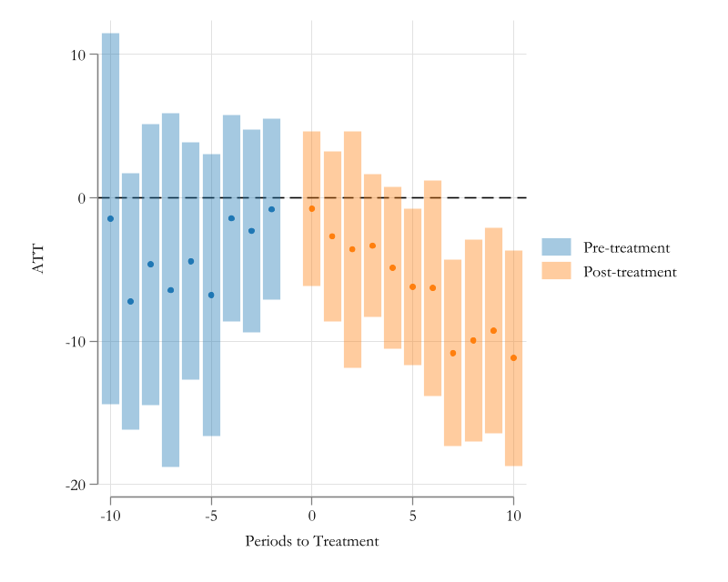
Advantage of csdid2 over other methods. Uniform Confidence Intervals using Wildbootstrap SE.

Conclusions

• In this workshop I aimed to provide a brief overview of the problems with TWFE and the potential solutions.
• 3 main solutions were presented:
  1. Avoid using bad controls (Borusyak, Jaravel, and Spiess (2023) and Gardner (2022))
  2. Allow for heterogeneity in the treatment effect. (Wooldridge (2021) and Sun and Abraham (2021))
  3. Use only good DID designs. (Callaway and Sant’Anna (2021))

Conclusions

• All methods have their own advantages and disadvantages.
• 3. is the most robust based on the assumptions, but is the least efficient because of the sample size requirements. It also allows for flexiblity of DR estimators, and ensures you use pre-treatment controls only.
• 1. and 2) are more efficient, (more data is used), but rely strongy on Long PTA assumption.
• 2. can be applied in non-linear settings, using nonlinear models. But aggregations are slower to obtain.
• 1. and 2) can also be adapted to consider -dose-response- effects. As well as Treatment Reversals.

Thank you!

Comments? Questions?

Suggested readings

Borusyak, Kirill, Xavier Jaravel, and Jann Spiess. 2023. “Revisiting Event Study Designs: Robust and Efficient Estimation.” https://arxiv.org/abs/2108.12419.

Caetano, Carolina, and Brantly Callaway. 2022. “Difference-in-Differences with Time-Varying Covariates in the Parallel Trends Assumption.” https://doi.org/10.48550/ARXIV.2202.02903.

Callaway, Brantly, and Pedro H. C. Sant’Anna. 2021. “Difference-in-Differences with Multiple Time Periods.” Journal of Econometrics, Themed Issue: Treatment Effect 1, 225 (2): 200–230. https://doi.org/10.1016/j.jeconom.2020.12.001.

Chaisemartin, Clément de, and Xavier D’Haultfœuille. 2020. “Two-Way Fixed Effects Estimators with Heterogeneous Treatment Effects.” American Economic Review 110 (9): 2964–96. https://doi.org/10.1257/aer.20181169.

———. 2023. “Two-Way Fixed Effects and Differences-in-Differences with Heterogeneous Treatment Effects: A Survey.” The Econometrics Journal 26 (3): C1–30. https://doi.org/10.1093/ectj/utac017.

Gardner, John. 2022. “Two-Stage Differences in Differences.” https://arxiv.org/abs/2207.05943.

Goodman-Bacon, Andrew. 2021. “Difference-in-Differences with Variation in Treatment Timing.” Journal of Econometrics 225 (2): 254–77. https://doi.org/https://doi.org/10.1016/j.jeconom.2021.03.014.

Roth, Jonathan, Pedro H. C. Sant’Anna, Alyssa Bilinski, and John Poe. 2023. “What’s Trending in Difference-in-Differences? A Synthesis of the Recent Econometrics Literature.” Journal of Econometrics 235 (2): 2218–44. https://doi.org/10.1016/j.jeconom.2023.03.008.

Sant’Anna, Pedro H. C., and Jun Zhao. 2020. “Doubly Robust Difference-in-Differences Estimators.” Journal of Econometrics 219 (1): 101–22. https://doi.org/10.1016/j.jeconom.2020.06.003.

Sun, Liyang, and Sarah Abraham. 2021. “Estimating Dynamic Treatment Effects in Event Studies with Heterogeneous Treatment Effects.” Journal of Econometrics, Themed Issue: Treatment Effect 1, 225 (2): 175–99. https://doi.org/10.1016/j.jeconom.2020.09.006.

Wooldridge, Jeffrey M. 2021. “Two-Way Fixed Effects, the Two-Way Mundlak Regression, and Difference-in-Differences Estimators.” SSRN Journal. https://doi.org/10.2139/ssrn.3906345.

———. 2023. “Simple Approaches to Nonlinear Difference-in-Differences with Panel Data.” The Econometrics Journal 26 (3): C31–66. https://doi.org/10.1093/ectj/utad016.