(NLSW, 1988 extract)
(211 real changes made)

grade -- Current grade completed
-----------------------------------------------------------
              |      Freq.    Percent      Valid       Cum.
--------------+--------------------------------------------
Valid   11    |        334      14.87      14.88      14.88
        12    |        943      41.99      42.02      56.91
        13    |        176       7.84       7.84      64.75
        14    |        187       8.33       8.33      73.08
        15    |         92       4.10       4.10      77.18
        16    |        252      11.22      11.23      88.41
        17    |        106       4.72       4.72      93.14
        18    |        154       6.86       6.86     100.00
        Total |       2244      99.91     100.00
Missing .     |          2       0.09
Total         |       2246     100.00
-----------------------------------------------------------Math Refresher
Basic Statistics and Probability
Random Variables
- A random variable is a variable whose value is determined by the outcome of a random experiment.
- For example, if we toss a coin, the outcome is random, but the possible values of \(X\) are 0 and 1.
- If we roll a die, the outcome is random with possible values 1, 2, 3, 4, 5, and 6.
- Exact temperature in a room
There are two kinds of random variables:
- Discrete random variables can only take on a finite number of values. For example, the number of heads in 10 coin tosses is a discrete random variable.
- The probability of observing a particular value is not always zero
- Continuous random variables can take on any value in a range. For example, the height of a randomly selected person is a continuous random variable.
If \(X\) is discrete random variable, then \(P(X=c)\) is the probability that \(X\) takes on the value \(c\). It can be any value between 0 and 1. ()
By definition, the sum of all probabilities for all feasible values of \(X\) is 1. That is, \(\sum_{c} P(X=c)=1\).
If \(X\) is continuous random variable, then \(P(X=c)=0\) for any value \(c\).
- The probability to observe a particular number is zero.
- Instead, when using continuous data, we focus on the probability of observing a value in a range. For example, \(P(1.7 \leq X \leq 1.8)\) is the probability that \(X\) is between 1.7 and 1.8, which can be any value between 0 and 1.
Stata and Random Variables
- Computers CANNOT generate random numbers. They can only generate pseudo-random numbers.
- Random numbers cannot be reproduced.
- Pseudo-random numbers can be reproduced, if we know initial conditions. (seed)
- For most purposes, pseudo-random numbers are good enough.
Statahas many built-in function to generate random numbers.help randomfor more information.
Probability Distributions
- A probability distribution is a function that assigns probabilities to the values of a random variable.
- For discrete random variables, we can use a table to describe the probability distribution. For example, the probability distribution of the number of heads in 5 coin tosses is:
| Number of heads | Probability |
|---|---|
| 0 | 0.03125 |
| 1 | 0.15625 |
| 2 | 0.3125 |
| 3 | 0.3125 |
| 4 | 0.15625 |
| 5 | 0.03125 |
In this case, the sum of all probabilities is 1.
Probability Density Functions
- For continuous random variables, we can use a function to describe the probability distribution.
- For example, we can say that the probability distribution of the height of a randomly selected person is:
\[f(x)\]
This function has important properties:
- \(f(x) \geq 0\) for all \(x\).
- \(\int_{-\infty}^{\infty} f(x) dx = 1\).
- \(P(a \leq X \leq b) = \int_{a}^{b} f(x) dx\).
- \(P(X \leq a) + P(X > a) = 1\).
- \(P(a \leq X \leq b) = P(X < b) - P(X < a)\).
Stata and Empirical Distributions
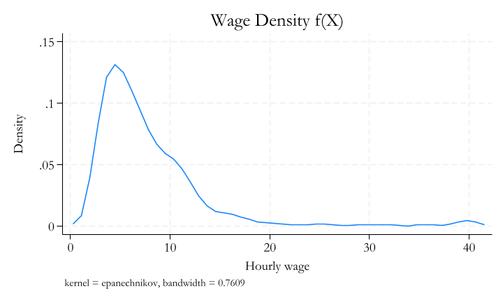
- Given a dataset, you can use different tools to estimate the probability distribution or the probability density function of a random variable.
- For example, you can use histograms, or frequency tables, to estimate the probability distribution of a discrete random variable.
- You can use kernel density plots to estimate the probability density function of a continuous random variable.
Joint Probability Distributions
The joint probability distribution of \(X\) and \(Y\) is a function that assigns probabilities to the values of \(X\) and \(Y\).
For discrete random variables, we can use a table to describe the joint probability distribution.
           |        Married
      Race |    Single    Married |     Total
-----------+----------------------+----------
     White |     21.68      51.20 |     72.89
     Black |     13.76      12.20 |     25.96
     Other |      0.36       0.80 |      1.16
-----------+----------------------+----------
Total | 35.80 64.20 | 100.00 - It must be the case that the sum of all probabilities is 1.
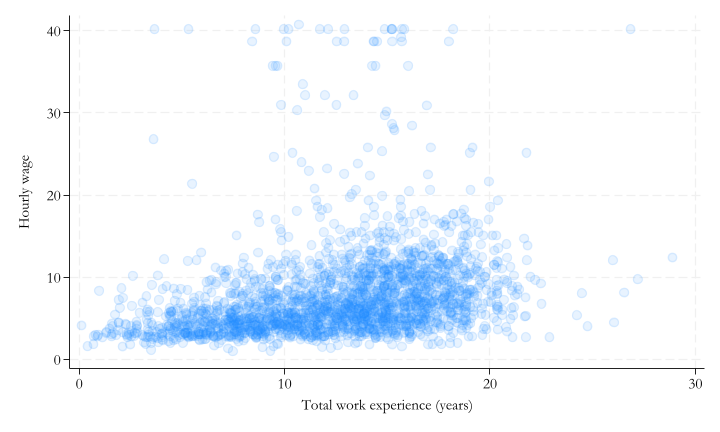
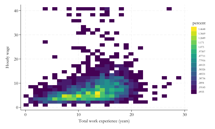
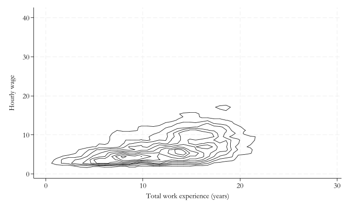
For continuous variables, estimation and graphical representation is tricky
it must be the case that:
\[\int_{-\infty}^{\infty} \int_{-\infty}^{\infty} f(x,y) dx dy = 1\]
- You may be able to use scatter plots, or contour plots, to represent the joint probability distribution of two continuous random variables.
Conditional Probability
The conditional probability of \(X\) given \(Y\) is:
\[P(x|y) = \frac{P(x,y)}{P(y)}\]
or, the conditional probabilty density function:
\[f(x|y) = \frac{f(x,y)}{f(y)}\]
And if \(X\) and \(Y\) are independent, then:
\(P(x|y) = P(x)\) or \(f(x|y) = f(x)\).
Marginal Probability Distributions
The marginal probability distribution of \(X\) is the probability distribution of \(X\) ignoring/regardless the values of \(Y\). This can be expressed as:
\[P(x) = \sum_{z=-\infty}^{\infty} P(X=x,y=z) \text{ or } f_x(x) = \int_{z=-\infty}^{\infty} f(x,z)dz\]
This is also refer to “integrating out” the variable \(Y\) or averaging over \(Y\).
\[P(x) = \sum_{z=-\infty}^{\infty} P(X=x|y=z)P_y(z) \text{ or } f_x(x) = \int_{z=-\infty}^{\infty} f(x|z)f_y(z)dz\]
Independence
Two random variables \(X\) and \(Y\) are independent if and only if:
\[P(x,y) = P(x)P(y) \text{ or } f(x,y)=f(x)*f(y)\]
That means the conditional probability of \(X\) given \(Y\) is the same as the marginal probability of \(X\).
\(P(x|y) = P(x)\) or \(f(x|y) = f(x)\).
Summary Statistics
Given a random variable \(X\), there are several summary statistics that can be used to describe the distribution of \(X\), without describing the entire distribution
Central Tendency
- Mean: average value of \(X\).
\[\bar x = E(X) = \sum_{x} xP(X=x) \text{ or } E(X) = \int_{-\infty}^{\infty} xf(x)dx\]
- Median: middle value of \(X\).
- Percentile: values that identify the boundaries of the distribuion. Median is the 50th percentile.
\[Q_y(p) = E(Y \leq Q_y) = p\]
- Mode: most frequent value of \(X\).
sum var,d in Stata will give you the mean, median, and selected quantiles.
mode can be estimated using egen, or based on empirical distribution.
Dispersion
- Variance: Average squared deviation from the mean.
\[Var(X) = E(X-\mu)^2 = \sum_{x} (x-\mu)^2P(X=x) \text{ or } Var(X) = \int_{-\infty}^{\infty} (x-\mu)^2f(x)dx\]
Standard deviation: square root of the variance. Easier to interpret.
Range: difference between the maximum and minimum values of \(X\).
Interquartile range: difference between the 75th and 25th percentiles of \(X\).
sum var,d and tabstat can provide you with most of this information.
Some useful distributions
Discrete distributions
- Bernoulli distribution: \(X \sim Bernoulli(p)\), where \(p \in [0,1]\).
- \(E(X)=p\) and variance \(Var(X)=p(1-p)\).
- Flip a coin with probability \(p\) of getting heads.
rbinomial(1, p)
- Binomial distribution: \(X \sim Binomial(n,p)\), where \(p \in [0,1]\) and \(n>0\)
- \(E(x)=np\) and \(Var(X)=np(1-p)\).
- Distribution of the number of successes in \(n\) independent Bernoulli trials.
rbinomial(n, p)
- Poisson distribution: \(X \sim Poisson(\lambda)\), where \(\lambda>0\)
- \(E(X)=Var(x)=\lambda\), Typically used for counts.
- For example, the number of customers arriving at a store in a given hour.
rpoisson(lambda)
Continuous distributions
- Uniform distribution: \(X \sim Uniform(a,b)\)
- \(f(x)=\frac{1}{b-a}\) for \(a \leq x \leq b\), and \(f(x)=0\) otherwise.
- \(E(X)=\frac{a+b}{2}\) and \(Var(X)=\frac{(b-a)^2}{12}\).
runiform(a, b)
- Normal distribution: \(X \sim Normal(\mu,\sigma^2)\)
- \(f(x)=\frac{1}{\sqrt{2\pi\sigma^2}}e^{-\frac{(x-\mu)^2}{2\sigma^2}}\).
- \(E(X)=\mu\) and \(Var(X)=\sigma^2\).
rnormal(mu, sigma)
Other useful distributions include:
- t-distribution, Chi-squared distribution, F-distribution
help density_functionshelp random_number_functions


