Regression Analysis I

Simple Regression

Fernando Rios-Avila

Levy Economics Institute

October 16, 2024

Regression

  • Regression is the most widely used method of comparison in data analysis.
  • Doing so uncovers the pattern of association between \(y\) and \(x\). Here, it is important what you use as \(y\) or \(x\).
  • Simple regression uncovers mean-dependence between two variables.
    • It amounts to comparing average values of one variable, called the dependent variable (\(y\)), for observations that are different in the other variable, the explanatory variable (\(x\)).
  • Multiple regression analysis involves more variables -> for later.

Regression - uses

  • Discovering patterns of association between variables is often a good starting point even if our question is more ambitious.
  • Causal analysis: uncovering the effect of one variable on another variable. Concerned with one parameter.
  • Predictive analysis: what to expect of a \(y\) variable (long-run polls, hotel prices) for various values of another \(x\) variable (immediate polls, distance to the city center).

Regression - names and notation

  • Regression analysis is a method that uncovers the average value of a variable \(y\) for different values of another variable \(x\).

\[\mathbb{E}[y|x]=y^E = f(x)\]

  • dependent variable or left-hand-side variable, or simply the \(y\) variable,
  • explanatory variable, right-hand-side variable, or simply the \(x\) variable
  • “regress y on x,” or “run a regression of y on x” = do simple regression analysis with \(y\) as the dependent variable and \(x\) as the explanatory variable.

Regression - type of patterns

Regression may find:

  • Linear patterns: positive (negative) association - average \(y\) tends to be higher (lower) at higher values of \(x\).
  • Non-linear patterns: association may be even non-monotonic - \(y\) tends to be higher for higher values of \(x\) in a certain range of the \(x\) variable and lower for higher values of \(x\) in another range of the \(x\) variable
  • No association or relationship (A flat line)

Non-parametric and parametric regression

  • Non-parametric regressions describe the \(\mathbb{E}[y] = f(x)\) pattern without imposing a specific functional form on \(f\).
  • Data driven and flexible, no theory
  • Can capture any pattern
  • Parametric regressions impose a functional form on \(f\). Parametric examples include:
    • linear functions: \(f(x) = a + bx\);
    • exponential functions: \(f(x) = a x^b\);
    • quadratic functions: \(f(x) = a + bx + cx^2\),
    • or any functions which have parameters of a, b, c, etc.
  • Restrictive, but they produce readily interpretable numbers.

Non-parametric regression: average by each value

  • Non-parametric regressions come (also) in various forms.
  • Most intuitive non-parametric regression for \(\mathbb{E}[y|x] = f(x)\) shows average \(y\) for each and every value of \(x\).
  • Works well when \(x\) has few values and there are many observations in the data,
  • There is no functional form imposed on \(f\) here.

Non-parametric regression: Categorical variable

  • Sometimes, there are no straightforward functional form on \(f\) (linear not meaningful).
    • Categorical variables
    • Ordered variables.
  • For example, Hotels: average price of hotels with the same numbers of stars and compare these averages = non-parametric regression analysis.

Non-parametric regression: bins

  • With many \(x\) values therea are two ways to do non-parametric regression analysis: bins and smoothing.
  • Bins - based on grouped values of \(x\) (Discretization of \(x\))
    • Bins are disjoint categories (no overlap) that span the entire range of \(x\) (no gaps).
  • Many ways to create bins - equal size, equal number of observations per bin, or bins defined by analyst.
    • see binscatter or make your own

Non-parametric regression: lpoly

  • Produce “smooth” graph - both continuous and has no kink at any point.
  • also called smoothed conditional means plots = non-parametric regression shows conditional means, smoothed to get a better image.
  • Lowess = most widely used non-parametric regression methods that produce a smooth graph.
  • locally weighted scatterplot smoothing (sometimes abbreviated as “loess”).
  • A smooth curve fit around a bin scatter.
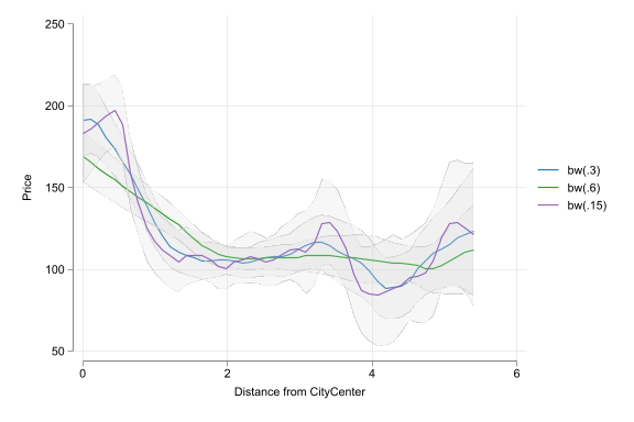
  • wider bandwidth results in a smoother graph but may miss important details of the pattern.
  • narrower bandwidth produces a more rugged-looking graph
  • In Stata one of the commands for this its lpoly but also lowess.

Non-parametric regression: lowess (loess)

  • Smooth non-parametric regression methods, including lowess, do not produce numbers that would summarize the \(\mathbb{E}[y]|x = f(x)\) pattern.
  • Provide a value \(\mathbb{E}[y]\) for each of the particular \(x\) values that occur in the data, as well as for all \(x\) values in-between.
  • Graph – we interpret these graphs in qualitative, not quantitative ways.
  • They can show interesting shapes in the pattern, such as non-monotonic parts, steeper and flatter parts, etc.
  • Great way to find relationship patterns

Case Study: Finding a good deal among hotels

Code
set scheme white2
color_style tableau
use data_slides/hotels-vienna.dta, clear
qui:drop if distance>6
two (lpolyci price distance, bw(.3) fcolor(%20)) ///
(lpolyci price distance, bw(.6) fcolor(%20)) ///
(lpolyci price distance, bw(.15) fcolor(%20)), ///
legend(order(2 "bw(.3)" 4 "bw(.6)" 6 "bw(.15)")) ///
ytitle("Price") xtitle("Distance from CityCenter")

Linear regression

Linear regression

Linear regression is the most widely used method in data analysis.

  • Imposes linearity assumption of the function \(f\) in \(\mathbb{E}[y|x] = f(x)\). (Linearity of Coefficients)
  • Linear functions have two parameters, also called coefficients: the intercept and the slope. \(\mathbb{E}[y|x] = \alpha + \beta x\)
  • Can be any function, including any nonlinear function, of the original variables themselves
  • This line is the best-fitting line one can draw through the scatterplot.
  • It is the best fit in the sense that it is the line that is closest to all points of the scatterplot.

Linear regression - assumption vs approximation

  • Assumption: The regression function is linear in its coefficients.
  • Approximation: Whatever the form of the \(\mathbb{E}[y|x] = f(x)\) the \(\mathbb{E}[y|x] = \alpha + \beta x\) regression fits a line through it.
    • This may or may not be a good approximation.

Linear regression coefficients

\[\mathbb{E}[y|x] = \alpha + \beta x\]

Two coefficients:

  • intercept: \(\alpha =\) average value of \(y\) when \(x\) is zero:
    • \(\mathbb{E}[y|x=0] = \alpha + \beta \times 0 = \alpha\).
  • slope: \(\beta =\) expected difference in \(y\) corresponding to a one unit difference in x.
    • \(\mathbb{E}[y|x=x_0+1] - \mathbb{E}[y|x_0] = (\alpha + \beta \times (x_0 + 1)) - (\alpha + \beta \times x_0) = \beta\).

Regression - slope coefficient interpretation

Several good ways to interpret the slope coefficient

  • \(y\) is \(\beta\) higher, on average, for observations with a one-unit higher value of \(x\).
  • Comparing two observations that differ in \(x\) by one unit, we expect \(y\) to be \(\beta\) higher for the observation with one unit higher \(x\).

Avoid using

  • “decrease/increase” – not right, unless time series or causal relationship only
  • “effect” – not right, unless causal relationship

Regression: binary \(x\)

Simplest case:

  • \(x\) is a binary variable, zero or one.
  • \(\alpha\) is the average value of \(y\) when \(x\) is zero (\(\mathbb{E}[y|x=0] = \alpha\)).
  • \(\beta\) is the difference in average \(y\) between observations with \(x=1\) and observations with \(x=0\)
    • \(\mathbb{E}[y|x=1] - \mathbb{E}[y|x=0]= \beta\).
  • Graphically, the regression line of linear regression goes through two points: average \(y\) when \(x\) is zero (\(\alpha\)) and average \(y\) when \(x\) is one (\(\alpha + \beta\)).

Regression coefficient formula

Notation

  • Population coefficients are \(\alpha\) and \(\beta\).

  • Sample estimates - \(\hat{\alpha}\) and \(\hat{\beta}\)

  • The slope coefficient formula is \[\hat{\beta} = \frac{\text{Cov}[x, y]}{\text{Var}[x]} = \frac{\sum_{i=1}^n (x_i - \bar{x})(y_i - \bar{y})}{\sum_{i=1}^n (x_i - \bar{x})^2} \]

  • Slope coefficient formula is normalized version of the covariance between \(x\) and \(y\).

Regression coefficient formula

  • The intercept – average \(y\) minus average \(x\) multiplied by the estimated slope \(\hat{\beta}\). \[\hat{\alpha} = \bar{y} - \hat{\beta} \bar{x} \]

  • The formula of the intercept reveals that the regression line always goes through the point of average \(x\) and average y.

Ordinary Least Squares (OLS)

  • The formulas Provided for the slope and intercept can be found using OLS (an estimation method).
  • OLS gives the best-fitting linear regression line.
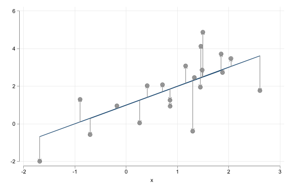
  • It gives the best line by minimizing the squared of the model errors.
Code
clear 
qui:set obs 20
qui:gen x = rnormal()+1
qui:gen y = 1+x+rnormal()
qui:gen yh=1+x
two (scatter y x, msize(3) mcolor(gs3%50)) ///
   (line yh x, color(navy)) (pcarrow yh x y x, color(gs9)), ///
legend(off)

Regression coefficient formula

  • Ordinary Least Squares – OLS is method used to find the best fit minimizing the Squared “residuals”.

    \[\min_{\alpha,\beta} \sum_{i=1}^n (y_i - \alpha - \beta x_i)^2\]

For this minimization problem, we can use calculus to give \(\hat{\alpha}\) and \(\hat{\beta}\), the values for \(\alpha\) and \(\beta\) that give the minimum. Please check out U7.1.

Recap

  • Simple regression analysis amounts to comparing average values of a dependent variable (\(y\)) for observations that are different in the explanatory variable (\(x\)).
  • Simple regression in any way or form: comparing conditional means.

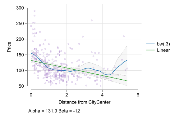
Case Study: Finding a good deal among hotels

Code
use data_slides/hotels-vienna.dta, clear
qui:drop if distance>6
qui: keep if inrange(stars,3,4)
qui: drop if price>300
two (lpolyci price distance, bw(.3) fcolor(%20)) ///
(lfitci price distance, fcolor(%20)) ///
(scatter price distance, color(%20)), ///
legend(order(2 "bw(.3)" 4 "Linear" )) ///
ytitle("Price") xtitle("Distance from CityCenter") ///
scale(1.4) note(Alpha = 131.9 Beta = -12)

Predictions and Residuals

Predicted values

  • The predicted value of the dependent variable is the best guess for its average value, given \(x\), using our model.
  • In a linear regression they are given by: \(\hat{y} = \hat{\alpha} + \hat{\beta}x\)
  • What about non-parametric regressions
    • It depends on how the Model was estimated.

Residuals

  • The residual is the difference between the actual value and predicted value of an observation: \(e_i = y_i - \hat{y}_i\), where \(\hat{y}_i = \hat{\alpha} + \hat{\beta}x_i\)

  • The residual is meaningful only for actual observation, cannot be “predicted” out of sample.

  • But, The residual may be important on its own right.

  • May help in identifying Outliers: Cases where \(y\) is much higher or much lower than “it should be” (based on the regression). (Good deals or places to avoid)

Case Study: Finding a good deal among hotels

Code
qui:drop2 pr_hat res
qui:reg price distance
qui:predict pr_hat
qui:predict res, res
qui:sort res
list hotel_id price distance pr_hat res star in 1/5
variable pr_hat not found
variable res not found

     +------------------------------------------------------------+
     | hotel_id   price   distance     pr_hat         res   stars |
     |------------------------------------------------------------|
  1. |    22080      54        1.1   118.6571   -64.65714       3 |
  2. |    22122      59         .8   122.2709    -63.2709       3 |
  3. |    21912      60        1.1   118.6571   -58.65714       4 |
  4. |    22073      59        1.2   117.4525   -58.45255       3 |
  5. |    22127      58        1.4   115.0434   -57.04337     3.5 |
     +------------------------------------------------------------+

Not the best model (functional form , other characteristics), but a good start!

Regression modelling

Regression modelling: \(R^2\)

  • Fitness of a regression captures how predicted values compare to the actual values.

  • R-squared (R^2) represents how much of the variation in \(y\) is captured by the regression, and how much is left for residual variation \[R^2 = \frac{\text{Var}[\hat{y}]}{\text{Var}[y]} = 1 - \frac{\text{Var}[e]}{\text{Var}[y]} \]

  • This follows: \[\text{Var}[y] = \text{Var}[\hat{y}] + \text{Var}[e]\]

Model fit - R^2

  • R-squared (or R^2) can also be identified for non-parametric regressions. \[R^2_1 = \frac{\text{Var}[\hat{y}]}{\text{Var}[y]} \text{ or } R^2_2= 1 - \frac{\text{Var}[e]}{\text{Var}[y]} \]
    • They may not be the same!
  • You could also estimate it using the “Squared correlation” between \(y\) and \(\hat y\).
  • The value of R-squared is always between zero and one.
  • R-squared is zero, if the predicted values are just the average of the observed outcome \(\hat{y}_i = \bar{y}_i\), \(\forall i\).

Model fit - how to use \(R^2\)

  • R-squared may help in choosing between different versions of regression for the same data.
    • Choose between regressions with different functional forms
    • Predictions are likely to be better with high \(R^2\)
    • More on this later
  • R-squared matters less when the goal is to characterize the association between \(y\) and \(x\)

Regression vs Causation

Regression and causation

  • Up to this point, try to be very careful to use neutral language, not talk about causation
  • Think back to sources of variation in \(x\)
  • When we have observational data, and we pick \(x\) and \(y\) and decide how to run the regression
  • Regression is a method of comparison: it compares observations that are different in variable \(x\) and shows corresponding average differences in variable \(y\). Not necessarily Causal Relations.

Regression and causation - possible relations

  • Slope of the \(\mathbb{E}[y|x] = \alpha + \beta x\) regression is not zero in our data
  • Several reasons, not mutually exclusive:
    • \(x\) causes \(y\): Yay!
    • \(y\) causes \(x\). Noo!
    • A third variable causes both \(x\) and \(y\) (or many such variables do) Double NoO!
  • In reality if we have observational data, there is a mix of these relations.

Regression and causation

  • Yes: “correlation (regression) does not imply causation”
    • Better: we should not infer cause and effect from comparisons in observational data.
  • Suggested approach is two steps
    • First interpret precisely the object (correlation of slope coefficient)
    • Conclude and discuss causal claims if any

Case Study: Finding a good deal among hotels

  • Fit and causation
  • The R-squared of the regression is 0.10 = 10%.
  • There is a lot left unexplained.
    • Still, good for cross-sectional regression with a single explanatory variable.
    • In any case it is the fit of the best-fitting line.

Case Study: Finding a good deal among hotels

  • Slope is -12
  • Does that mean that a longer distance causes hotels to be cheaper?

Summary take-away

  • Regression – method to compare average \(y\) across observations with different values of \(x\).
  • Non-parametric regressions (bin scatter, lowess, lpoly): use them to visualize complicated patterns of association between \(y\) and \(x\), No Number to interpret.
  • Linear regression – linear approximation of the average pattern of association \(y\) and \(x\)
  • When \(\beta\) is not zero, one of three things (+ any combination) may be true:
    • \(x\) causes y
    • \(y\) causes x
    • A third variable causes both \(x\) and y

Break!

Regression Analysis II

Complicated Patterns (not everything is straight)

Motivation

  • Interested in the pattern of association between life expectancy in a country and how rich that country is.
    • Uncovering that pattern is interesting for many reasons: discovery and learning from data.
  • Identify countries where people live longer than what we would expect based on their income, or countries where people live shorter lives.
  • Analyzing regression residuals.
  • Getting a good approximation of the \(y_E = f(x)\) function is important.

Functional form

Functional form

  • So far, we have only considered linear regression. (aside from non-parametric regressions)
  • Relationships between \(y\) and \(x\) are often complicated!
  • When and why care about the shape of a regression?
    • When we need to talk about the non-average person.
  • How can we capture function form better?
    • We can transform variables in a simple linear regression.

Functional form - linear approximation

  • Linear regression is a linear approximation to a regression of unknown shape:

  • But, we may want to modify the regression to better characterize nonlinear patterns

    • prediction or analyze residuals - better fit
    • we want to go beyond the average pattern of association (different \(x\)s)
    • all we care about is the average pattern of association, but the linear approximation is bad
  • Not care

    • if all we care about is the average pattern of association,
    • if linear regression is good approximation to the average pattern

Functional form - types

Non linearities can be captured in many ways: - Natural log transformation: \(\ln(x)\) when interested in relative differences - Piecewise linear splines: For flexibility in the pattern of association - Polynomials - quadratic form: Flexible yet simple

log transformation

  • Some times, some patterns are better approximated when \(y\) or \(x\) are measured as relative differences
    • Particularly relevant if there is no natural base for comparison.
  • Taking the natural logarithm of a variable is often a good solution in such cases, because they approximate relative differences.

Logarithmic transformation - interpretation

  • \(\ln(x)\) or \(\log(x)\) is the natural logarithm of \(x\)

    • You can only use it if \(x\) is always a positive number
    • \(\ln(0)\) or \(\ln(\text{negative number })\) are not \(Real\)
  • Using this transformation, you can compare relative differences: \[\ln(x + \Delta x) - \ln(x) \approx \frac{\Delta x}{x}\]

  • as long as \(\Delta x\) is small.

    • \(\ln(1.01)-\ln(1) = 0.0099 \approx 0.01\)
    • \(\ln(1.1)-\ln(1) = 0.095 \approx 0.1\)
    • but…\(\ln(1.4)-\ln(1) = 0.336\) much less than 0.4

When to take logs?

  • When comparison makes mores sense in relative terms
    • Percentage differences, relative differences, growth rates
  • Most important examples
    • Prices
    • Sales, turnover, GDP
    • Population, employment
    • Capital stock, inventories

Interpreting parameters of regressions with log variables

\(\ln(y^E) = \alpha + \beta x_i\)

  • log \(y\), level \(x\)
  • \(\alpha\) is average \(\ln(y)\) when \(x\) is zero. (Often meaningless.)
  • \(\beta\): \(y\) is \(\beta * 100\) percent higher, on average for observations with one unit higher \(x\).

\(y^E = \alpha + \beta\ln(x_i)\)

  • level \(y\), log \(x\)
  • \(\alpha\) is : average \(y\) when \(\ln(x)\) is zero (and thus \(x\) is one), not very meaningful.
  • \(\beta\): \(y\) is \(\beta/100\) units higher, on average, for observations with one percent higher \(x\).

\(\ln(y^E) = \alpha + \beta\ln(x_i)\)

  • log \(y\), log \(x\)
  • \(\alpha\): is average \(\ln(y)\) when \(\ln(x)\) is zero. (Often meaningless.)
  • \(\beta\): \(y\) is \(\beta\) percent higher on average for observations with one percent higher \(x\).
    • Elasticity!
  • Precise interpretation is key
  • The interpretation of the slope (and the intercept) coefficient(s) differs in each case!
  • Often verbal comparison is made about a 10% difference in \(x\) if using level-log or log-log regression.
To Take log or Not to Take log

Decide for substantive reason:

  • Take logs if variable is likely affected in multiplicative ways
  • Don’t take logs if variable is likely affected in additive ways

Decide for statistical reason:

  • Linear regression is better at approximating average differences if distribution of dependent variable is closer to normal.
  • Take logs if skewed distribution with long right tail
  • Most often the substantive and statistical arguments are aligned

To Take log or Not to Take log

  • Log needs variable to be positive: Never negative, never zero
  • Sometimes you may be able to combine Logs with Dummies (if zero or negative values are present)
  • Sometimes adding a constant seems to do the trick
    • \(\ln(x+1)\) if \(x\) is positive or zero
    • But Not a good solution. May need to consider other transformations

Hotel price-distance regression and functional form

Comparing different models

Code
qui {
  set linesize 255
  capture gen log_price = log(price)
  capture gen log_distance = log(distance)
  regress price distance
  est sto m1
  regress log_price distance
  est sto m2
  regress price log_distance
  est sto m3
  regress log_price log_distance
  est sto m4
}
esttab m1 m2 m3 m4, se md nostar nonumber note("")
price log_price price log_price
distance -12.05 -0.104
(2.001) (0.0161)
log_distance -21.28 -0.176
(2.251) (0.0183)
_cons 131.9 4.829 114.8 4.682
(3.740) (0.0301) (2.087) (0.0169)
N 321 321 320 320

As Excercise, plot the different models.

Which model shall we choose? - Substantive reasons

  • It depends on the goal of the analysis!
  • Prices
    • We are after a good deal on a single night – absolute price differences are meaningful.
    • Percentage differences in price may remain valid if inflation and seasonal fluctuations affect prices proportionately.
    • Or we are after relative differences - we do not mind about the magnitude that we are paying, we only need the best deal.
  • Distance
    • Distance could make more sense in miles than in relative terms – given our purpose is to find a relatively cheap hotel.

Which model shall we choose? - Statistical reasoning

  • Visual inspection
    • Which model captures patterns better?
  • Compare fit measure (\(R^2\))
    • But be careful. If \(y\) is in logs, \(R^2\) is not directly comparable to \(R^2\) when \(y\) is in levels.
    • its like comparing apples and oranges
  • Final verdict:
    • Your call….

Making things MORE flexible

Other transformations: splines

  • Warning Splines are another way to estimate non-parametric models. Just a bit more parametric.
  • A regression with a piecewise linear spline (of \(x\)) results in connected line segments for the mean dependent variable,
    • each line segment corresponding to a specific interval of the explanatory variable.
  • The points of connection are called knots,
  • The places of the knots (the boundaries of the intervals of the explanatory variable) need to be specified by the analyst.
  • Plot-twist: The segments need not to be linear!

Other transformations: splines

  • Advantage: We can interpret parameters!
  • The formula:

\[y^E = \alpha_1 + \beta_1 x[\text{if } $x$ < k_1] + (\alpha_2 + \beta_2 x)[\text{if } k_1 \leq $x$ \leq k_2] + \dots + (\alpha_m + \beta_m x)[\text{if } $x$ \geq k_{m-1}]\]

But we we usually assume that \(\alpha_2, \alpha_3, \dots, \alpha_m = 0\) and only allow \(\beta's\) to change

Other transformations: splines

Interpretation of the most important parameters

  • \(\alpha\): average \(y\) when \(x\) is zero.
  • \(\beta_1\): How much higher \(y\) is, on average, for observations with one unit higher \(x\) value, if \(x \in (-\infty , k_1)\).
  • \(\beta_2\): How much higher \(y\) is, on average, for observations with one unit higher \(x\) value, if \(x \in (k_2, k_2)\).
  • Etc. This is the “slope” of the line segment.
  • You can also use marginal slopes.

Splines - Example

  • You need to create all necessary variables, given your knots.
  • Say we choose knots 1 and 2 for the price analysis
*              v Knot  v knot2
mkspline dist1 1 dist2 2 dist3= distance  
Code
regress price dist1 dist2 dist3

      Source |       SS           df       MS      Number of obs   =       321
-------------+----------------------------------   F(3, 317)       =     41.08
       Model |  162850.558         3  54283.5192   Prob > F        =    0.0000
    Residual |  418846.994       317  1321.28389   R-squared       =    0.2800
-------------+----------------------------------   Adj R-squared   =    0.2731
       Total |  581697.551       320  1817.80485   Root MSE        =    36.349

------------------------------------------------------------------------------
       price | Coefficient  Std. err.      t    P>|t|     [95% conf. interval]
-------------+----------------------------------------------------------------
       dist1 |  -75.91485   8.747817    -8.68   0.000    -93.12596   -58.70373
       dist2 |  -.1596926   7.344118    -0.02   0.983    -14.60907    14.28968
       dist3 |    2.54916   3.843377     0.66   0.508     -5.01259    10.11091
       _cons |   174.5939   6.098417    28.63   0.000     162.5954    186.5924
------------------------------------------------------------------------------

Other transformations: splines

  • Splines can handles any kind of nonlinearity
  • Offers a lot of flexibility,
  • But requires decisions from the analyst
    • How many knots?
    • Where to locate them
    • Decision based on scatterplot, theory / business knowledge
    • Machine learning
  • They can also be more complicated: quadratic, cubic or B-splines. Smooth and flexible.

Polynomials

This is a simpler way to capture non-linearities

  • Quadratic function of the explanatory variable, allowing for a smooth change in the slope
    • Technically: quadratic function is not a linear function (a parabola, not a line), but the model is still linear in its coefficients.
  • Handles nonlinearities similar to a parabola.
  • Less flexible, but easier interpretation!
    • Just need basic calculus, or “logic”

The quadratic form

\[y^E = \alpha + \beta_1 x + \beta_2 x^2\]

  • \(\beta_1\) has no interpretation (unless x=0),
  • \(\beta_2\neq 0\) if the functional form is U-shaped (\(\beta_2 > 0\)) or inverted U-shaped (\(\beta_2 < 0\)).
    • But you may not see it in the data
  • The slope: \(\beta_1 + 2\beta_2 x\) is different at different values of \(x\).
  • You can use slope for comparing the effect of \(x\) on \(y\) for small changes in \(x\).
  • For large changes, need to calculate manually.

Life expectancy and income

  • Is there a relationship between How long people live in a country and how rich that country is?
  • To identify countries where people live longer than what we would expect based on their income, or countries where people live shorter lives.
  • Analyzing regression residuals – getting a good approximation of the \(y_E = f(x)\) function is important.

Life expectancy and income

use data_slides/wb-lifeexpectancy.dta, clear
keep if year == 2017
sum gdppc lifeexp
(4,847 observations deleted)

    Variable |        Obs        Mean    Std. dev.       Min        Max
-------------+---------------------------------------------------------
       gdppc |        182    19.22786    20.38674   .6707771   113.2622
     lifeexp |        182    72.30765    7.648017     52.214   84.68049

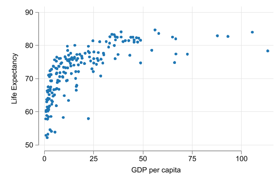
Life expectancy and GDP

Code
scatter lifeexp gdppc, scale(1.4) ///
ytitle(Life Expectancy) xtitle(GDP per capita) ///
xlabel(0(25)100)

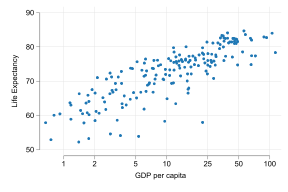
Code
scatter lifeexp gdppc, scale(1.4) ///
ytitle(Life Expectancy) xtitle(GDP per capita) ///
xscale(log) xlabel(1 2 5 10 25 50 100)

gen log_gdp = log(gdppc)
regress lifeexp log_gdp
predict resid, res
predict life_hat
sort resid

      Source |       SS           df       MS      Number of obs   =       182
-------------+----------------------------------   F(1, 180)       =    382.77
       Model |  7200.86382         1  7200.86382   Prob > F        =    0.0000
    Residual |  3386.21735       180  18.8123186   R-squared       =    0.6802
-------------+----------------------------------   Adj R-squared   =    0.6784
       Total |  10587.0812       181  58.4921612   Root MSE        =    4.3373

------------------------------------------------------------------------------
     lifeexp | Coefficient  Std. err.      t    P>|t|     [95% conf. interval]
-------------+----------------------------------------------------------------
     log_gdp |   5.333648   .2726172    19.56   0.000     4.795712    5.871585
       _cons |   59.65933   .7220205    82.63   0.000     58.23462    61.08404
------------------------------------------------------------------------------
(option xb assumed; fitted values)
list countryname lifeexp gdppc life_hat if inrange(_n,1,5) | inrange(_n,178,182) 

     +---------------------------------------------------+
     |       countryname   lifeexp      gdppc   life_hat |
     |---------------------------------------------------|
  1. | Equatorial Guinea    57.939   22.29894   76.21785 |
  2. |           Nigeria    53.875   5.351441   68.60581 |
  3. |          Eswatini    58.268   9.567586   71.70473 |
  4. |     Cote d'Ivoire    54.102   3.564596   66.43867 |
  5. |           Lesotho    54.568   2.845889   65.23766 |
     |---------------------------------------------------|
178. |           Lebanon    79.758   11.64702    72.7537 |
179. |           Vietnam    76.454   6.233485   69.41956 |
180. |           Vanuatu    72.334    2.82708   65.20229 |
181. |         Nicaragua    75.653   5.169298   68.42111 |
182. |   Solomon Islands    71.006   2.126353   63.68308 |
     +---------------------------------------------------+

Life expectancy and income: Can we do better?

  • Probably…Linear regression seems a good fit, but you can try other functional forms.
    • Quadradic, Splines, etc
  • Keep \(y\) is the same for easy comparison
    • Explore the residuals, see if you can do better.

Which functional form to choose? - guidelines

Start with deciding whether you care about nonlinear patterns or not.

  • Linear approximation OK if focus is on an average association.
  • Transform variables for a better interpretation of the results (e.g. log), and it often makes linear regression better approximate the average association.
  • Accommodate a nonlinear pattern if our focus is
    • on prediction,
    • analysis of residuals,
    • about how an association varies beyond its average.
  • Keep in mind - simpler the better!

See you Next Class

Messy data

Measurement error!
Extreme values! and influential observations! Not everything is as it seems

Data Is Messy

  • Clean and neat data exist only in dreams, and textbooks
  • Data may be messy in many ways
    • Structure, storage type differs from what we want
    • Needs cleaning (see Chapters 1,2)
    • Some observations are influential
    • Variables measured with error
    • Some observations may represent more individuals (Weights?)

Extreme values

  • Some observations may contain Extreme values, compared to the rest of the data
  • Extreme values examples
    • Banking sector employment share in countries. Luxembourg: 10%
    • Hotel price of 1 US dollars, 10,000 US dollars
    • Production of a small firm: 1,000,000,000 units

Influential observations

  • Influential observations
    • Their inclusion or exclusion influences the regression line (sensitivity)
    • Influential observations are often extreme values (on \(x\) or \(y\))
    • But not all extreme values are influential observations
  • Influential observations example
    • Very large tech companies in a regression of size and average wage
    • A single mixed-race worker in a regression

What to do with them?

  • Depends on why they are extreme
  • If by mistake: may want to drop them (EUR1000+) (or Impute them)
  • If by nature: don’t want to drop them (Part of the distribution)
  • Grey zone: patterns work differently for them for substantive reasons
  • General rule: avoid dropping observations based on value of \(y\) variable
    • Dropping extreme observations by \(x\) variable may be OK
    • But those are valuable as they represent informative and large variation

Measurement Errors In Variables

  • Goal: measuring the association between variables
    • Furthermore, we are interested in the estimated value (not just the sign)
  • But, observed variables have measurement error
    • Mistake, hard-to-measure data, created variables
  • Often cannot do anything about it!
  • So, what the consequence is of such errors??
  • Does the answer depend on the type of measurement error?

Classical Measurement Error

\[w = w^* + \varepsilon\]

  1. is zero on average (so it does not affect the average of the measured variable) and
  2. is independent of all other relevant variables, including the error-free variable.
  • Recording errors: E.g., due to mistakes in entering data
  • Reporting errors: in surveys or administrative data If they are random around the true quantities

CME in the dependent variable (\(y\))

Consider \(y = y^* + e\), where \(y\) is the measured variable, \(y^*\) is the error-free variable, and \(e\) is the measurement error (noise).

The slope coefficient of \(y\) and \(y^*\) on \(x\) are:

\[\beta^* = \frac{\text{Cov}[y^*, x]}{\text{Var}[x]} \text{ and } \beta = \frac{\text{Cov}[y^* + e, x]}{\text{Var}[x]} \]

\[\beta = \frac{\text{Cov}[y^*, x]}{\text{Var}[x]} + \left(\frac{\text{Cov}[e, x]}{\text{Var}[x]}\approx 0\right) \approx \beta^* \]

  • Consequence: classical measurement error in \(y\) is not expected to affect the regression coefficients.

CME in the explanatory variable (\(x\))

Consider \(x = x^* + e\), where \(x\) is the measured variable, \(x^*\) is the error-free variable, and \(e\) is the measurement error (noise).

The slope coefficient are: \[\beta^* = \frac{\text{Cov}[y, x^*]}{\text{Var}[x^*]} \text{ and } \beta = \frac{\text{Cov}[y, x^*+e]}{\text{Var}[x^*+e]} \]

\[\beta = \frac{\text{Cov}[y, x^*]+(\text{Cov}[y, e]\approx 0)}{\text{Var}[x^*]+\text{Var}[e]} = \beta^* \frac{\text{Var}[x^*]}{\text{Var}[x^*]+\text{Var}[e]} \]

  • Consequence: CME in \(x\) will affect the regression coefficients. (Towards zero) Attenuation Bias
  • \(\alpha\) is also affected

Classical measurement error in the explanatory variable (\(x\))

  • Noise to signal ratio is: \(\frac{\text{Var}[e]}{\text{Var}[x^*]}\)
    • How much noise is there compared to the true variation \(x*\)
  • When the noise-to-signal ratio is low, we may safely ignore the problem.
    • this happens often when
      • when we are confident that recording errors are at not important
      • when our data has an aggregate variable estimated from very large samples.
  • When the noise-to-signal ratio is substantial
    • we may be better of assessing its consequences.

Extra: non-classical measurement error

  • In real-life data measurement error in variables may or may not be classical
    • Very often, it isn’t!
  • Variables measured with error may be less dispersed (non-zero mean)
    • Example: Self reported Income
  • Measurement error may be related to variables of interest
    • Example: Self-reported weight and height
  • This often means that modelling needs to be redesigned

Classical measurement error summary

  1. CME in the dependent (\(y\)) variable is not expected to affect the regression coefficients.
  2. CME in the explanatory (\(x\)) variable will affect the regression coefficients.
    1. The estimated beta will be closer to zero than it would be without measurement error.
  3. Almost all variables are measured with error. Need to think about consequences.

Hotel ratings and measurement error

  • Review the case of Ratings and Prices of hotels
    • Average customer ratings are noisy and bad proxies for the true quality of a hotel.
    • The true quality of a hotel is unobserved.
  • Regressions for hotels with few ratings are likely to produce attenuated slope coefficients.
  • And that is what you can find!
    • I would argue the same with Amazon reviews
  • But what to do?
    • perhaps Robustness checks. Restrict regressions to cases with different levels of Measurement error.

Using weights in regressions

  • Different observations may have different weights (importance or size)
    • to denote different size of larger units in the data
    • population of countries
  • Use weights of size IF want to uncover the patterns of association for the individuals
    • who make up the larger units (e.g., people in countries),
  • Also, use weights when you want your data to be representative of the population
    • when you want to generalize the results to the population

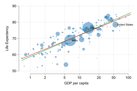
Life expectancy and GDP per capita - weights

Code
qui: reg lifeexp log_gdp [w=population ]
predict life_hatw
qui: reg lifeexp log_gdp 
predict life_hatnw
*p*redict life_hat
two (scatter lifeexp gdppc [w=population ],  color(%50)) ///
(scatter lifeexp gdppc [w=population ] if inlist(countryname,"China","India","United States"),  color(%50) mlabel(countryname)) ///
(line life_hatw life_hatnw gdppc,sort  ), scale(1.4) legend(off) ///
ytitle(Life Expectancy) xtitle(GDP per capita) ///
xscale(log) xlabel(1 2 5 10 25 50 100)
(option xb assumed; fitted values)
(analytic weights assumed)

Summary take-away

  • Nonlinear functional forms may or may not be important for regression analysis.
  • They are usually important for prediction.
  • less important for causal analysis.
  • When important, we have multiple options: Logs, splines, polynomials
  • Influential observations and other extreme values are usually best analyzed with the rest of the data
  • Discard them only if you have a good reason.

Regression Analysis III

Generalizing Regression Results Hypothesis Testing 2.0

Regressions and Statistical Inference

Generalizing: reminder

  • We have uncovered some pattern in our data. We are interested in generalize the results.
  • Question: Is the pattern we see in our data
    • True in general?
    • or is it just a special case (unique to the sample)?
  • Inference - the act of generalizing results
    • From a particular dataset to other situations.
  • From a sample to population = statistical inference
  • Beyond (other dates, countries, people, firms) = external validity

Generalizing Linear Regression

  • We estimated the linear model
    • \(\hat{\beta}\) is the average difference in \(y\) in the dataset between observations that are different in terms of \(x\) by one unit.
    • \(\hat{y}_i\) best guess for the expected value (average) of the dependent variable for observation \(i\) with value \(x_i\)
  • Sometimes all we care about patterns in the data we have.
  • But often we are interested in patterns beyond the Dataset.
  • To what extent they can be generalized

Statistical Inference: Confidence Interval

  • The 95% CI of the slope coefficient is similar to estimating a 95% CI of any other statistic. \[CI(\hat{\beta})_{95\%} = [\hat{\beta} - 1.96SE(\hat{\beta}), \hat{\beta} + 1.96SE(\hat{\beta})] \]

  • The standard error (SE) of the slope coefficient

    • is conceptually the same as the SE of any statistic.
    • measures the spread of the values of the statistic across hypothetical repeated samples drawn from the same population our data represents

Standard Error of the Slope

\[SE(\hat{\beta}) = \frac{Std[e]}{\sqrt n Std[x]}\]

  • Where:
    • Residual: \(e = y - \hat{\alpha} - \hat{\beta}x\)
    • \(Std[e]\), the standard deviation (SD) of the regression residual,
    • \(Std[x]\), the SD of the explanatory variable,
    • \(\sqrt{n}\) , Often we use \(\sqrt{n - 2}\).
  • A smaller standard error translates into narrower CI and more precise estimates.
  • We get more precision if
    • smaller the standard deviation of the residual (better fit)
    • larger the standard deviation of the explanatory variable – more variation in \(x\) is good.
    • more data.
  • This formula is correct assuming homoskedasticity

Heteroskedasticity Robust SE

  • Simple SE formula is not correct in general.

  • Homoskedasticity assumption, the goodness of fit of the regression line is the same across the entire range of the \(x\) variable.

    • Residuals are spread evenly around the regression line.
  • In general this is not true

  • Heteroskedasticity: the fit may differ at different values of \(x\) so that the spread of actual \(y\) around the regression is different for different values of \(x\)

  • So…what to do?

    • Need to adjust the SE formula!

Heteroskedasticity: You have options

  • There are many ways to correct for heteroskedasticity
    • Generalized least squares (GLS)
    • Weighted least squares (WLS)
    • Feasible generalized least squares (FGLS)
    • Huber-White robust standard errors
  • Traditionally, you also want to test if you have a Heteroskedasticity problem
    • White test, Breusch-Pagan test

But for now lets assume you have a heteroskedasticity problem

Heteroskedasticity Robust SE

  • White-Huber Robust SE is correct with and without heteroskedasticity.
  • Same properties as before: smaller when \(Std[e]\) is small, \(Std[x]\) is large and \(n\) is large
  • Mathematically, Huber-White SE “corrects” the simple SE using the residuals from the regression. \[Var_r(\hat{\beta}) = \frac{\sum (x_i-\bar x)^2 \hat e_i^2}{\left(\sum (x_i-\bar x)^2\right)^2}\]

Note: there are many heteroskedastic-robust formula: ‘HC0’, ‘HC1’, ‘HC2’, ‘HC3’. Stata uses HC1 when you ask for robust SE: regress y x, robust

Anythings else?

  • Nope
    • Coefficient and \(R^2\) remain the same
  • Just make sure you are using robust SE.
  • SE may be similar, but most likely larger than the simple SE

Testing if (true) beta is zero

  • Testing hypotheses: decide if a statement about a general pattern is true.

  • The question: are the Dependent variable and the explanatory variable related at all?

  • The null and the alternative: \[H_0: \beta_{true} = 0, H_A: \beta_{true} \neq 0\]

  • The t-statistic is: \[t = \frac{\hat{\beta} - 0}{SE(\hat{\beta})}\]

  • Often \(t = 2\) (1.96) is the critical value, which corresponds to 95% CI. or 5% significance level (\(\alpha\)) \((t = 2.6 \rightarrow 99\%)\)

Testing if (true) beta is zero

Practical guidance, Same as before!:

  • Choose a critical value.
    • p-value, the probability of a false positive in our dataset
    • Balancing act: false positive (FP) and negative (FN)
  • Higher critical value
    • FP: less likely (less likely rejection of the null).
    • FN: more likely (high risk of not rejecting a null even though it’s false)
  • Typical critical values: 5% (1.96)

Ohh, that \(p=5\%\) cutoff

  • When testing, you start with a critical value first
  • Often the standard to publish a result is to have a p value below 5%.
    • Arbitrary, but…there is lots of discussion about it.
  • If you find a result that cannot be told apart from 0 at 1% (max 5%), you should say that explicitly.
    • Sometimes that is what you want to say. A non-significant result is also a result.

Dealing with 5-10%

  • Sometimes regression result may be significant at 10%.
  • What not to do? Avoid language like…
    • “a barely detectable statistically significant difference” (\(p=0.073\))
    • “a margin at the edge of significance” (\(p=0.0608\))
  • Sometimes you work on a proposal: Proof of concept.
    • To be lenient is okay. You may need more power!
    • Say the point estimate and note the 95% confidence interval.
  • Sometimes you are looking for a proof. Beyond reasonable doubt.
    • Here you wanna be below 1% (or less)
    • Be honest…present the p-value, and the CI.

p-Hacking

  • Just as before. Be honest. Do not fixate on the 5% level.

Suggestion:

  • Present your most conservative result first
    • Example: if uncertain, keep extreme values in.
  • Show robustness checks: many additional regressions with different decisions

Chance Events And Size of Data

  • Some times you just need more power.
  • Finding patterns by chance may go away with more observations
  • Specificities to a single dataset may be less important if more sources
  • More observations help only if
    • Errors and idiosyncrasies affect some observations but not all
    • Additional observations are from appropriate source
    • If worried about specificities of Vienna more observations from Vienna would not help

Prediction and Uncertainty

Prediction uncertainty

  • Goal: predicting the value of \(y\) for observations outside the dataset, when only the value of \(x\) is known.

  • We predict \(y\) based on coefficient estimates, which are relevant in the general pattern/population. With linear regression you have a simple model: \[y_i = \hat{\alpha} + \hat{\beta}x_i + \epsilon_i \]

  • The estimated statistic here is a predicted value for a particular observation \(\hat{y}_j\). For an observation \(j\) with known value \(x_j\) this is \[\hat{y}_j = \hat{\alpha} + \hat{\beta}x_j\]

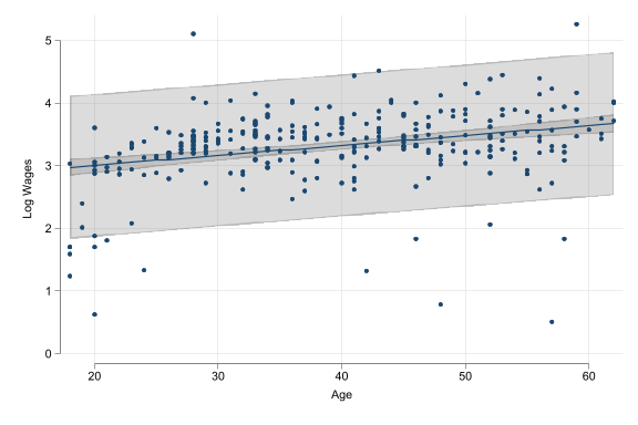
Prediction uncertainty

  • You can produce two kinds of intervals:
    • Confidence interval for the predicted value/regression line
      • Uncertainty comes from \(\hat{\alpha}, \hat{\beta}\)
    • Prediction interval, uncertainty comes from \(\hat{\alpha}, \hat{\beta}\) and \(\epsilon_i\)

Confidence interval of the regression line I.

  • The predicted value \(\hat{y}_j\) is based on \(\hat{\alpha}\) and \(\hat{\beta}\) only.

    • Thus, the CI of the predicted value combines the CI for \(\hat{\alpha}\) and the CI for \(\hat{\beta}\).
  • What to expect if we know the value of \(x_j\) and \(\hat{\alpha}\) and \(\hat{\beta}\)?.

    \[95\%CI(\hat{y}_j) = \hat{y_j} \pm 1.96 SE(\hat{y}_j)\]

  • The standard error of the predicted value is \[SE(\hat{y}_j) = \frac{Std[e]}{\sqrt{\frac{1}{n}+ \frac{(x_j - \bar{x})^2}{nVar[x]}}} \]

  • Use robust SE formula in practice, but a simple formula is instructive

Prediction interval

  • Prediction interval answers:
    • Where to expect the particular \(y_j\) value if we know the corresponding \(x_j\) value and the estimates of the regression coefficients?
  • The CI of the predicted value is about \(\hat{y}_j\): Where would the average value of the dependent variable be if we know \(x_j\).
  • The PI (prediction interval) is about \(y_j\) itself not its average value, what range of values we expect for \(y_j\) if we know \(x_j\).
  • So PI starts with CI. But adds additional uncertainty (\(Std[\epsilon_i]\)) that actual \(y_j\) will be around its conditional.

Prediction interval

  • The formula for the 95% prediction interval is
    • \(95\%PI(\hat{y}_j) = \hat{y} \pm 1.96SPE(\hat{y}_j)\)
    • \(SPE(\hat{y}_j) = Std[e]\sqrt{\textbf{1} + \frac{1}{n} + \frac{(x_j - \bar{x})^2}{nVar[x]}}\)
  • SPE – Standard Prediction Error (SE of prediction)
  • Summarizes the additional uncertainty: the actual \(y_j\) value is expected to be spread around its average value.
    • This is best estimated by the standard deviation of the residual \(e\).
  • In the formula, all elements get very small if \(n\) gets large, except for the new element.

Prediction interval

Code
qui:ssc install frause,
qui:frause oaxaca, clear
qui: drop if runiform()<.8 
qui: sort age
qui: reg lnwage age
qui: predict lnwage_hat
qui: predict se_ci, stdp
qui: predict se_pi, stdf
qui: gen ci_low = lnwage_hat - 1.96*se_ci
qui: gen ci_up = lnwage_hat + 1.96*se_ci
qui: gen pi_low = lnwage_hat - 1.96*se_pi
qui: gen pi_up = lnwage_hat + 1.96*se_pi
twoway  (rarea pi_low pi_up age, color(gs5%25) ) ///
(rarea ci_low ci_up age, color(gs5%25) ) ///
       (scatter lnwage age, color(navy)) (line lnwage_hat age, color(navy)) ///
       , legend(off) ytitle(Log Wages) xtitle(Age)

External validity

External validity

  • Statistical inference helps us generalize to the population or general pattern
  • Is this true beyond the data (other dates, countries, people, firms)?
    • we can’t assess it using our data.
  • We’ll never really know. Only think, investigate, make assumption, and hope…

However…

  • Analyzing other data can help!
  • Focus on \(\beta\), the slope coefficient on \(x\).
  • The three common dimensions of generalization are: time, space, and other groups.
  • To learn about external validity, we always need additional data, on say, other countries or time periods.
  • We can then repeat regression and see if slope is similar!
  • Meta-analysis: combining results from different studies to learn about external validity.

Stability of hotel prices - idea

  • Here we ask different questions: whether we can infer something about the price–distance pattern for situations outside the data:
    • Is the slope coefficient close to what we have in Vienna, November, weekday:
      • Other dates (we will do this)
      • Other cities
      • Other type of accommodation: apartments
    • Compare them to our benchmark model result

Benchmark model

  • The benchmark model is a spline with a knot at 2 miles.
  • Dependent variable: log price
  • Data is restricted to 2017, November weekday in Vienna, 3-4 star hotels, within 8 miles.

Comparing dates

2017-NOV-weekday 2017-NOV-weekend 2017-DEC-holiday 2018-JUNE-weekend
dist_0_2 -0.31 -0.44 -0.36 -0.31
(0.038) (0.052) (0.041) (0.037)
dist_2_7 0.02 0.00 0.07 0.04
(0.033) (0.036) (0.050) (0.039)
Constant 5.02 5.51 5.13 5.16
(0.042) (0.067) (0.048) (0.050)
Observations 207 125 189 181
R.squared 0.314 0.430 0.382 0.306

Note: Robust standard errors in parentheses *** p<0.01, ** p<0.05, * p<0.1

  • November weekday and the June weekend: \(\hat{\beta}_1 = -0.31\)
  • Estimate is similar for December (-0.36 log units)
  • Different for the November weekend: they are 0.44 log units or 55% (exp(0.44) - 1) cheaper during the November weekend.
    • The corresponding 95% confidence intervals overlap somewhat: they are [-0.39,-0.23] and [-0.54,-0.34].
    • Thus we cannot say for sure that the price–distance patterns are different during the weekday and weekend in November.

Stability of hotel prices - takeaway

  • Fairly stable overtime but uncertainty is larger
  • Evidence of some external validity in Vienna
  • External validity – if model applied beyond data, there is additional uncertainty!

Take-away

  1. Regression Fundamentals: Regression analysis is essential for identifying relationships between variables. It’s used for both causal and predictive analysis.

  2. Coefficient Interpretation: In linear regression, the intercept and slope have specific meanings, indicating the expected values and changes in the dependent variable relative to the explanatory variable.

  3. Non-linear Relationships: Non-linear patterns can be captured using non-parametric methods and transformations like logs and splines. Depends on the goal of the analysis.

  4. Data Challenges: Real-world data issues like measurement errors and extreme values can affect regression results. Analysts must carefully manage these challenges.

  5. Generalization and Inference: Statistical inference helps generalize findings beyond the sample, but external validity requires additional data and context.

Reading-Homework

Read Case Study as an example of a simple linear regression analysis.