Modeling Probabilities

to be or not to be

Fernando Rios-Avila

Levy Economics Institute

August 26, 2024

What we will see today

Linear Probability Model - LPM
Logit & probit
Goodness of fit
Diagnostics
Summary

Motivation

What are the health benefits of not smoking? Considering the 50+ population, we can investigate if differences in smoking habits are correlated with differences in health status.
- good health vs bad health

Binary events

Some outcomes are things that either happen or don’t happen, which can be captured by binary variables
- e.g. a person is healthy or not, a person is employed or not, a person is a smoker or not. We dont see a person that is half healthy, half employed, or half a smoker.
How can we model these events?
- We have seen this before. Instead of modeling the value itself, we model the probability of the event happening.

\[E[y] = P[y = 1]\]

In fact, the average of a 0–1 event is the probability of that event happening. Which can also be estimated as conditional probabilities:

\[E[y|x_1, x_2, ...] = P[y = 1|x_1, x_2, ...]\]

Good news, we can use the same tools we have been using to model these probabilities.

Modelling events: LPM

LPM: Linear probability model

Linear Probability Model (LPM) is a linear regression with a binary dependent variable
- It has the goal of modeling the probability of an event happening
A linear regressions with binary dependent variables shows:
- differences in expected \(y\) by \(x\), represent diferences in probability of \(y = 1\) by \(x\).
Introduce notation for probability: \(y^P = P[y = 1|x_1, x_2, . . .]\)
Linear probability model (LPM) regression is \(y^P = \beta_0 + \beta_1 x_1 + \beta_2 x_2\)

LPM: Interpretation

\[y^P = \beta_0 + \beta_1 x_1 + \beta_2 x_2\]

So far nothing changes in terms of modelling or estimation. However, the interpretation of the coefficients changes.
- \(y^P\) denotes the probability that the dependent variable is one, conditional on the right-hand-side variables of the model.
- \(\beta_0\) shows the predicted probability of \(y\) if all \(x\) are zero.
- \(\beta_1\) shows the difference in the probability that \(y = 1\) for observations that are different in \(x_1\) but are the same in terms of \(x_2\). (ceteris paribus)

LPM: Modelling

Linear probability model (LPM) can be estimated using OLS. (just like linear regression)
We can use all transformations in \(x\), that we used before:
- Log, Polinomials, Splines, dummies, interactions, etc. They all work.
All formulae and interpretations for standard errors, confidence intervals, hypotheses and p-values of tests are the same.
IMPORTANT Heteroskedasticity robust error are essential in this case!
- By construction LPMs are heteroskedastic!
- And ignoring this fact will lead to biased standard errors and confidence intervals.

LPM: Prediction

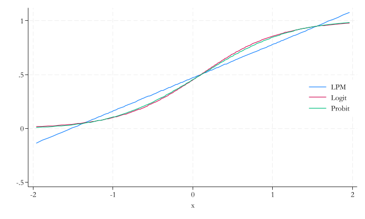
Predicted values - \(\hat{y}_P\) - may be problematic. Although they are calculated the same way, they need to be interpreted as probabilities.

\[\hat{y}^P = \hat{\beta}_0 + \hat{\beta}_1 x_1 + \hat{\beta}_2 x_2\]

Predicted values need to be between 0 and 1 because they are probabilities
But in LPM, predictions may be below 0 and above 1. No formal bounds in the model.
- more likely than certain, less likely than impossible

LPM: Prediction

When to get worried?:
- With continuous variables that can take any value (GDP, Population, sales, etc), this could be a serious issue (extrapolation)
  - We need to check if predictions are within the 0-1 range at least “in-sample”. But, this is not a guarantee that it will be the case “out-of-sample”.
- With binary variables, no problem (‘saturated models’) (interpolation)
  - Not problem because “simple” means will always be between 0 and 1.
So, a problem if goal is prediction!
Not a big issue for inference → uncover patterns of association.
- But it may give biased estimates…(in theory)

CS: Does smoking pose a health risk?

This is on of the few datasets from the book that is not directly available from their website. If interested, you need to go over the repository, and follow the instructions to access the data.

Thus, we will use a different dataset to illustrate the concepts.

CS: Does smoking during pregnancy affect birth weight?

The question is whether, and by how much, smoking during pregnancy affects the likelihood that a baby is born with low birth weight.
We will use “lbw” dataset from Stata’s example datasets.
The dataset contains information on 189 observations of mothers and their newborns.
- low is a binary variable indicating whether the baby was born with low birth weight (<2500gr <5.5lbs).
- smoke is a binary variable indicating whether the mother smoked during pregnancy.

Data

\(low = 1\) if baby was born with low birth weight
\(low = 0\) if baby was born with normal weight -Some demographic information on all individual
We exclude women <15 years old and >40 years old
Also exclude women with Weight > 200lbs (before pregnancy)

LPM: in Stata

Start with a simple univariate model: \(P[low|smoke] = \alpha + \beta[smoke]\)

webuse lbw, clear
drop if age < 15 | age > 40 | lwt > 200
reg low smoke, robust

(Hosmer & Lemeshow data)
(10 observations deleted)

Linear regression                               Number of obs     =        179
                                                F(1, 177)         =       4.70
                                                Prob > F          =     0.0316
                                                R-squared         =     0.0272
                                                Root MSE          =     .46208

------------------------------------------------------------------------------
             |               Robust
         low | Coefficient  std. err.      t    P>|t|     [95% conf. interval]
-------------+----------------------------------------------------------------
       smoke |    .157405   .0726412     2.17   0.032     .0140507    .3007593
       _cons |   .2568807   .0420845     6.10   0.000     .1738289    .3399326
------------------------------------------------------------------------------

LPM: Interpretation

Interpretation:

The coefficient on smoker shows the difference in the probability of a baby.
Babies are 15.7 percentage points more likely to be born with low birth weight if the mother smoked during pregnancy.
- Are you comparing Apples to apples?
- Lets add additional controls to capture other factors

LPM: with many regressors I

Multiple regression – closer to causality
Compare women who are very similar in many respects but are different in smoking habits
Smokers / non-smokers – different in many other behaviors and conditions:
- personal traits (age, race)
- behavior pre-pregnancy (Pre-pregnancy weight)
- Medical history (History of Hypertension)
- background for pregnancy (Number of prenatal visits, Previous premature labor)

LPM with many regressors II

May also consider functional form selection or interactions
Trial and error, or theory-based
Useful to check bivariate relationships (scatter plots, Lpoly, correlations)
- For now, assume linear relationships

LPM with many regressors III

Code

qui {
gen any_premature = ptl >0
ren ftv no_of_visits_1tr
ren ht hist_hyper
ren lwt wgt_bef_preg
reg low smoke age i.race any_premature hist_hyper  no_of_visits_1tr wgt_bef_preg, robust nohead
}
est store lpm_results
esttab lpm_results,   se  wide nonumber ///
collabel(b se) md drop(1.race) nomtitle b(3) nonotes

	b	se
smoke	0.151^*	(0.075)
age	-0.005	(0.007)
2.race	0.210	(0.112)
3.race	0.126	(0.079)
any_premature	0.275^**	(0.097)
hist_hyper	0.396^**	(0.143)
no_of_visits_1tr	-0.005	(0.034)
wgt_bef_preg	-0.002	(0.002)
_cons	0.464	(0.252)
N	179

Robust standard errors in parentheses ^* p < 0.05, ^** p < 0.01, ^*** p < 0.001

Detour: Regression Tables

If need to show many explanatory variables
Do not show table 12*2 rows, people will not see it.
- Avoid copy pasting from your document! Those tables are unwieldy.
Either only show selected variables (smoke + 2-3 others)
Or may need to create two columns. (a bit more work)
- In my case, Wide format did the trick.
Make site you have title, N of observations, footnote on SE, stars.
SE, stars: many different notations. Check carefully.
- esttab default is \(p^{***}= p<0.001\), \(0.01\) and \(0.05\)
- In papers there is \(p^{***}=p<0.01\), \(0.05\) and \(0.1\).

Does smoking pose a health risk for the baby?

Coefficient on smoking during pregnancy is -.151.
- Women who smoked during pregnancy are 15.1 percentage points more likely to have a baby with low birth weight.
The 95% confidence interval is relatively wide \([0.002, 0.300]\), but it does not contain zero
Age, Race?, Nr of Visits and Pre-pregnancy weight do not seem to be factors
Hypertension and previous premature labor are significant factors, increasing the probability of low birth weight by 40pp and 27.5pp, respectively.

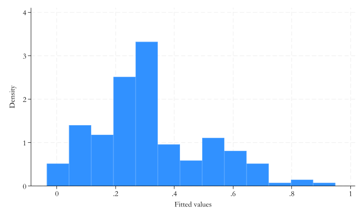
LPM’s predicted probabilities

Code

qui: reg low smoke age i.race any_premature hist_hyper  no_of_visits_1tr wgt_bef_preg, robust nohead
qui: predict low_hat
qui:histogram low_hat
sum low_hat


    Variable |        Obs        Mean    Std. dev.       Min        Max
-------------+---------------------------------------------------------
     low_hat |        179    .3184358    .1878437  -.0346098   .9483117

Analysis of LPM’s predicted probabilities

What to do
What we find

Drill down in distribution:
- Looking at the composition of people: top vs bottom part of probability distribution
- Look at average values of covariates for top and bottom X% of predicted probabilities!

Code

sort low_hat
set linesize 255
 
qui: gen flag = 1 if _n<=5
qui: replace  flag = 2 if _n>=_N-4
list low_hat smoke age race any_premature hist_hyper  no_of_visits_1tr wgt_bef_preg   if flag==1
list low_hat smoke age race any_premature hist_hyper  no_of_visits_1tr wgt_bef_preg   if flag==2


     +---------------------------------------------------------------------------------+
     |   low_hat       smoke   age    race   any_pr~e   hist_h~r   no_of_~r   wgt_be~g |
     |---------------------------------------------------------------------------------|
  1. | -.0346098   Nonsmoker    32   White          0          0          2        186 |
  2. | -.0280454   Nonsmoker    36   White          0          0          0        175 |
  3. |  .0019138   Nonsmoker    32   White          0          0          0        170 |
  4. |  .0158307   Nonsmoker    23   White          0          0          0        190 |
  5. |  .0284496   Nonsmoker    28   White          0          0          0        167 |
     +---------------------------------------------------------------------------------+

     +--------------------------------------------------------------------------------+
     |  low_hat       smoke   age    race   any_pr~e   hist_h~r   no_of_~r   wgt_be~g |
     |--------------------------------------------------------------------------------|
175. | .7197446      Smoker    34   Black          0          1          0        187 |
176. | .7369648   Nonsmoker    17   Black          0          1          0        142 |
177. | .8160616      Smoker    18   Black          1          0          0        110 |
178. | .8545191   Nonsmoker    26   Other          1          1          1        154 |
179. | .9483117   Nonsmoker    25   Other          1          1          0        105 |
     +--------------------------------------------------------------------------------+

Modelling events:
[log/prob]it

Probability models: logit and probit

Prediction: predicted probability need to be between 0 and 1
- Thus, for prediction, we must use non-linear models
- Actually, its a quasi-linear model.
The model, itself, is linear in the parameters
but need to relate this to the probability of the \(y = 1\) event, using a nonlinear function that maps the linear index into a 0-1 range: ‘Link function’

\[\begin{aligned} XB &= \beta_0 + \beta_1 x_1 + \beta_2 x_2 + ... \\ y^P &= F(XB) \rightarrow y^P \in (0,1) \end{aligned} \]

Two options: Logit and probit – different link function

Link functions I.

Call \(XB = \beta_0 + \beta_1 x_1 + \beta_2 x_2 + ...\)

The Logit:
\(y^P = \Lambda(XB) = \frac{\exp(XB)}{1 + \exp(XB)}\)
The probit:
\(y^P = \Phi(XB) \rightarrow \Phi(z) = \int_{-\infty}^z \frac{1}{\sqrt{2\pi}} \exp\left(-\frac{z^2}{2}\right) dz\)

where \(\Lambda()\) is called logistic function, and \(\Phi()\) is the cumulative distribution function (CDF) of the standard normal distribution.

Link functions II.

Both link functions are S-shaped curves bounded between 0 and 1.
There is but a small difference between the two.
but estimated coefficients will be different.

Code

qui {
clear
range p 0 1 202
drop if p==0 | p==1 
gen x = invnormal(p)
gen y = (x+rnormal())>0
reg  y x
predict y_1
logit y x
predict y_2
probit y x
predict y_3
drop if abs(x)>2
two (line y_1 x ) (line y_2 x) (line y_3 x), ///
legend(order(1 "LPM" 2 "Logit" 3 "Probit") pos(3) ring(0) col(1)) 
}

Logit and probit interpretation

Both the probit and the logit transform the \(\beta_0 + \beta_1 x_1 + ...\) linear combination using a link function that shows an S-shaped curve.
The slope of this curve keeps changing as we change whatever is inside, but it’s steepest when \(y^P = 0.5\) (inflection point)
The difference in \(y^P\) corresponds to changes in probabilities, between any two values of \(x\).
To find how much is related to a particular \(x\), You need to take the partial derivatives.
Important consequence: no direct interpretation of the raw coefficient values!
- Thus, always know if you are interpreting the raw coefficients or the marginal differences.

Marginal differences (marginal effects)

NOTE As before, the word “effect” should be used with caution. In the book, they use “marginal differences” instead. as a more neutral term.

Link functions makes associates \(\Delta x\) into \(\Delta y_P\). we do not interpret raw coefficients! (except for direction)
Instead, transform them into ‘marginal differences’ for interpretation purposes
They are also called ‘marginal effects’ or ‘average marginal effects (AME)’ or ‘average partial effects’.
Average marginal difference has the same interpretation as the coefficient of linear probability models, but with caveats.

Marginal differences: Discrete \(x\)

if \(x\) is a categorical (0-1), the marginal difference is the difference in the predicted probability of \(y = 1\), that corresponds to a change from \(x = 0\) to \(x = 1\).

\[\Delta y^P = y^P(x = 1) - y^P(x = 0)\]

Then we simply “average” this difference across all observations.

Marginal differences: continous \(x\)

If \(x\) is continuous, the marginal difference is calculated as the derivative (for a small change in \(x\)).

\[\frac{\partial y^P}{\partial x_1} = \beta_1 \cdot f(XB)\]

Which is then averaged across all observations to report a single number.
In practice, we interpret this as the change in the probability of \(y = 1\) for a one-unit change in \(x_1\).

How to estimate this models?

Maximum likelihood estimation!

When estimating a logit or probit model, we use ‘maximum likelihood’ estimation.
- See 11.U2 for details.
Idea for maximum likelihood is another way to get coefficient estimates.
- 1st You specify a (conditional) distribution, that you will use during the estimation.
  - This is logistic for logit and normal for probit model.
- 2nd You maximize this function w.r.t. your \(\beta\) parameters → gives the maximum likelihood for this model.
Different from OLS: No closed form solution → need to use search algorithms.
- Thus… more computationally intensive.

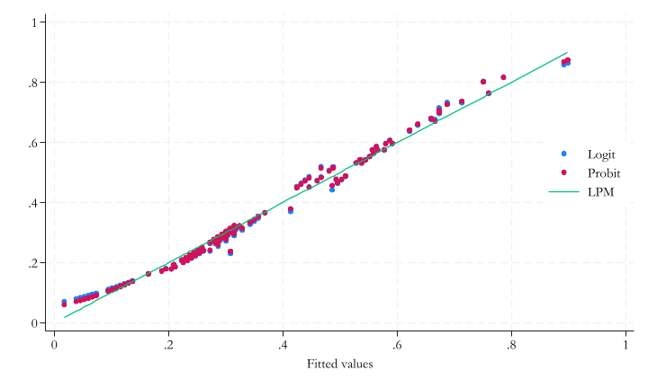
Predictions for LMP, Logit and Probit I.

Code

qui {
  webuse lbw, clear
  drop if age < 15 | age > 40 | lwt > 200
  gen any_premature = ptl >0
  ren ftv no_of_visits_1tr
  ren ht hist_hyper
  ren lwt wgt_bef_preg
  gen black = 2.race
  gen other = 3.race
  reg low smoke age i.black i.other i.any_premature hist_hyper , robust nohead
  predict low_hat_ols
  est sto lpm_results
  logit low smoke age black other any_premature hist_hyper , robust nohead
  predict low_hat_logit
   probit low smoke age black other any_premature hist_hyper , robust nohead
  predict low_hat_probit
   two (scatter  low_hat_logit low_hat_probit low_hat_ols) ///
      (line low_hat_ols low_hat_ols, sort), ///
      legend(order(1 "Logit" 2 "Probit" 3 "LPM") pos(3) ring(0) col(1))
}

Coefficient results for logit and probit

Code

qui {
  logit low smoke age i.black i.other i.any_premature hist_hyper , robust nohead
  est sto logit_results
  margins, dydx(*) post
  est sto logit_mfx
  probit low smoke age i.black i.other i.any_premature hist_hyper , robust nohead  
  est sto probit_results
  margins, dydx(*) post
  est sto probit_mfx
}
esttab lpm_results logit_results  logit_mfx probit_results probit_mfx, se  nonumber drop(0.*) ///
mtitle(LPM Logit Logit_MFX Probit Probit_MFX) collabel(none) md ///
star(* 0.10 ** 0.05 *** 0.01) nonotes

	LPM	Logit	Logit_MFX	Probit	Probit_MFX
main
smoke	0.166**	0.925**	0.169**	0.549**	0.169**
	(0.0739)	(0.397)	(0.0695)	(0.235)	(0.0697)
age	-0.00703	-0.0447	-0.00818	-0.0271	-0.00835
	(0.00669)	(0.0377)	(0.00688)	(0.0221)	(0.00679)
1.black	0.192*	1.012*	0.202*	0.607*	0.202*
	(0.111)	(0.526)	(0.109)	(0.314)	(0.108)
1.other	0.150*	0.884**	0.164**	0.524**	0.163**
	(0.0770)	(0.435)	(0.0787)	(0.254)	(0.0779)
1.any_premature	0.284***	1.330***	0.279***	0.810***	0.280***
	(0.0972)	(0.441)	(0.0944)	(0.270)	(0.0956)
hist_hyper	0.370***	1.720**	0.315***	1.063**	0.327***
	(0.137)	(0.674)	(0.117)	(0.415)	(0.122)
_cons	0.270	-0.971		-0.576
	(0.183)	(0.983)		(0.577)
N	179	179	179	179	179

Standard errors in parentheses ^* p < 0.1, ^** p < 0.04, ^*** p < 0.01

Does smoking pose a health risk?– logit and probit

LPM – interpret the coefficients as usual.
Logit, probit - Interpret the marginal differences. Basically the same.
- Marginal differences are essentially the same across the logit and the probit.
- Essentially the same as the corresponding LPM coefficients.
Happens often:
- Often LPM is good enough for interpretation.
- Check if logit/probit very different.
  - if so, Investigate functional forms if yes.

Goodness of fit measures

Goodness of fit

There is no generally accepted goodness of fit measure
- This is because we do not observe probabilities only 1 and 0, so we cannot FIT those probabilities.
There are, however, other options to evaluate the quality of the model.
- R-squared
- Brier score
- Pseudo R-squared
- log-loss

Goodness of fit: R-squared

\[R^2 = 1 - \frac{\sum_{i=1}^n (\hat{y}_P^i - y_i)^2}{\sum_{i=1}^n (y_i - \bar{y})^2}\]

R-squared is not useful for binary outcomes
- It can be calculated, but it lacks the interpretation we had for linear models, because we are fitting the probabilities, not the outcomes.

Brier score

\[\text{Brier} = \frac{1}{n}\sum_{i=1}^n (\hat{y}_P^i - y_i)^2\]

The Brier score is the average distance (mean squared difference) between predicted probabilities and the actual value of \(y\).
Smaller the Brier score, the better.
When comparing two predictions, the one with the smaller Brier score is the better prediction because it produces less (squared) error on average.
Related to a main concept in prediction: mean squared error (MSE)

Pseudo R2

\[pR^2 = 1 - \frac{\text{Log-likelihood}_{\text{model}}}{\text{Log-likelihood}_{\text{intercept only}}}\]

It is similar to the R-squared, as it measures the goodness of fit, tailored to nonlinear models and binary outcomes.
- Most widely used: McFadden’s R-squared (Stata uses this)
Computes the ratio of log-likelihood of the model vs intercept only.
Can be computed for the logit and the probit but not for the linear probability model. (unless you re-define the Log-likelihood)

Log-loss

\[\text{Log-loss} = \frac{1}{n}\sum_{i=1}^n \left[y_i \log(\hat{y}_P^i) + (1-y_i) \log(1-\hat{y}_P^i) \right]\]

The log-loss is a measured derived from the log-likelihood function. It measures how much observed data dissagrees with the predicted probabilities.
The smaller (close to zero) the log-loss, the better the model.

Practical use

There are several measured of model fit, but they often give the same ranking of models.
Do not use R-squared. Even for LPM, it has no interpretation.
If using probit vs logit: pseudo R-squared may be used to rank logit and probit models.
Use, especially for prediction: Brier score is a metric that can be computed for all models and is used in prediction.

Bias of the predictions

Post-prediction: we may be interested to study some features of our model
One specific goal: evaluating the bias of the prediction.
- Probability predictions are unbiased if they are right on average = the average of predicted probabilities is equal to the actual probability of the outcome.
- If the prediction is unbiased, the bias is zero.
Unless the model is really bad, unconditional bias is not a big issue.
- Only Probit will be biased.

Calibration

Unbiasedness refers to the whole distribution of probability predictions.
A finer and stricter concept is calibration
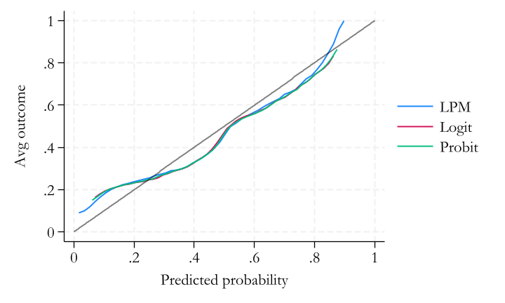
A prediction is well calibrated if the actual probability of the outcome is equal to the predicted probability for each and every value of the predicted probability. \[E(y|y^P) = y^P\]
‘Calibration curve’ is used to show this.
A model may be unbiased (right on average) but not well calibrated
- underestimate high probability events and overestimate low probability ones

Calibration curve

Horizontal axis shows the values of all predicted probabilities (\(\hat{y}_P\)).
Vertical axis shows the fraction of \(y = 1\) observations for all observations with the corresponding predicted probability.
The closer the curve is to the 45-degree line, the better the calibration.

In practice:

Create bins for predicted probabilities and make comparisons of the actual event’s probability.
Or use non-parametric methods to estimate the calibration curve.

Calibration curve

Code

two (lpoly low low_hat_ols) (lpoly low low_hat_logit) ///
(lpoly low low_hat_probit) (function y = x, range(0 1) lcolor(black%50)), ///
legend(order(1 "LPM" 2 "Logit" 3 "Probit") ) scale(1.5) ///
xtitle("Predicted probability") ytitle("Avg outcome")

Probability models summary

Find patterns when \(y\) is binary can be done using model probability with regressions
Linear probability model is mostly good enough, easy inference.
- to-go for data exploration, quick analysis, and diagnostics
- but, predicted values could be below 0, above 1
Logit (and probit) - better when aim is prediction, predicted values strictly between 0-1
Most often, LPM, logit, probit - similar inference
Use marginal (average) differences (with logit/probit)
No trivial goodness of fit. Brier score or pseudo-R-Squared.
Calibration is important for prediction.

Modeling Probabilities

What we will see today

Motivation

Binary events

Modelling events: LPM

LPM: Linear probability model

LPM: Interpretation

LPM: Modelling

LPM: Prediction

LPM: Prediction

CS: Does smoking pose a health risk?

CS: Does smoking during pregnancy affect birth weight?

Data

LPM: in Stata

LPM: Interpretation

LPM: with many regressors I

LPM with many regressors II

LPM with many regressors III

Detour: Regression Tables

Does smoking pose a health risk for the baby?

LPM’s predicted probabilities

Analysis of LPM’s predicted probabilities

Modelling events: [log/prob]it

Probability models: logit and probit

Link functions I.

Link functions II.

Logit and probit interpretation

Marginal differences (marginal effects)

Marginal differences: Discrete \(x\)

Marginal differences: continous \(x\)

How to estimate this models?

Maximum likelihood estimation!

Predictions for LMP, Logit and Probit I.

Coefficient results for logit and probit

Does smoking pose a health risk?– logit and probit

Goodness of fit measures

Goodness of fit

Goodness of fit: R-squared

Brier score

Pseudo R2

Log-loss

Practical use

Bias of the predictions

Calibration

Calibration curve

Calibration curve

Probability models summary

Modelling events:
[log/prob]it