Time series data

The past, the present, and the future

Fernando Rios-Avila

Levy Economics Institute

September 18, 2024

Motivation

  • You are considering investing in a company stock, and you want to know how risky that investment is. You have downloaded data on daily stock prices for many years. How should you define returns? How should you assess whether and to what extent returns on the company stock move together with market returns?

  • Heating and cooling are important uses of electricity. How does weather conditions affect electricity consumption? We are going to use monthly data on temperature and residential electricity consumption in Arizona. How to formulate a model which captures these factors?

What is special in the analysis of time series data?

Different

  • We have time series data if we observe one unit across many time periods.
  • There is a special notation: \(y_t\), \(t = 1, 2, \ldots, T\)
  • Time series data presents additional opportunities as well as additional challenges to compare variables.

With other features

  • Data wrangling novelties: frequency and aggregation
  • Special nature of time series: serial correlation
  • Coefficient interpretation.

Data preparation

  • What is Frequency? of time series? = time elapsed between two observations of a variable
  • Practical problems with frequency:
    • Not all data is captured at the same frequency
    • There may be regular/irregular gaps between them: e.g. weekends for stock-exchange
    • Two variables have different frequencies
    • Extreme values (spikes) in your variable
  • Last but not least: in Stata you need to Declare your data as time series data with tsset command

Consequences

  • Regressions: to condition \(y_t\) on values of \(x_t\) the two variables need to be on the same frequency. Otherwise, we need to adjust one of them.

  • How to adjust? Aggregation!

    • Flow variables: sum up the values within the interval. e.g. daily sales \(\rightarrow\) weakly sales is the sum of daily sales.
    • Stock variables: take the end-period value. e.g. daily stock prices uses the closing price on a given day
    • Other kinds of variables: usually take the average value

What is not special in time series

  • Time series regressions are special for several reasons…but many aspects remain the same

    • Generalization, confidence intervals: Same difficulties as in cross-section
    • Time series regression uncover patterns rather than evidence of causality: There is no “sample of time”
    • Practical data issues, missing observations, extreme values etc, remain
    • Coefficient interpretation is based on conditional comparison

What is special in time series

  • Ordering matters - key difference to cross section. Complications…Past before future
  • Trend - variables tend to have trends! Increasing or decreasing values over time
  • Seasonality - variables may show some cyclical component, such 4 seasons, months, - every e.g. December value is expected to be different.
  • Time series values are often not independent - correlated in time
    • Failure to account for this may lead to wrong (biased) conclusions

Properties

But they may also show Seasonality

  • There is seasonal variation, or seasonality, if its expected value changes periodically.
    • Follows the seasons of the year, days of the week, hours of the day.
  • Seasonality may be linear, when the seasonal differences are constant; it may be exponential, if relative differences (that may be approximated by log differences) are constant.
  • Important real life phenomenon - many economic activities follow seasonal variation over the year, through the week or day.
    • Thus they need to be accounted for in the analysis.

What is special in time series: Stationarity

To learn something, we need consistency in patterns If the patterns change constantly, we cannot learn anything from the data

  • Stationary time series have the same expected value and same distribution, at all times.
  • Stationarity is a feature of the time series itself.
  • Stationarity means stability (in expectations).
  • If series are stationary, we can learn from them!

What is special in time series: Non-stationarity

In absence of stationarity, we cannot learn anything from the data Or what we learn may be misleading

  • Non-stationary time series are those that are not stable for some reason.
  • Series that violate stationarity because the expected value is different at different times:
    • Has a trends
    • Has seasonality
    • Has some unstable patterns
  • Although, some of this issues can be address by “controlling” for them in the regression.

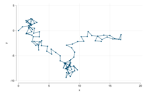
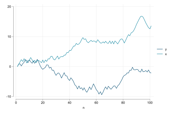
A Special case: Random walk

Some non-stationary variables are not easy to deal with:

  • Another example of non-stationary time series is the random walk.
  • Random walk when \(y_t\) follows a random walk if its value in \(t\) is the same as in \((t - 1)\) plus some random term: \(y_t = y_{t-1} + e_t\).
  • Time series variables that follow random walk change in completely random ways.
  • Whatever the previous change was the next one may be anything. Wherever it starts, a random walk variable may end up anywhere after a long time.

Code
qui: {
  clear
set scheme white2
color_style bay
qui:set obs 101
gen r = runiform(0,2*_pi)

gen y = 0 
gen x = 0
replace y = y[_n-1] + sin(r) if _n>1
replace x = x[_n-1] + cos(r) if _n>1
gen n = _n
}

*scatter  y x , connect(l) name(m1, replace) 
*line y x n, name(m2, replace) 

What to fear of Random walk

  • Random walks are impossible to predict
  • after a change, they don’t revert back to some value or trend line but continue their journey from that point.
  • Spread rising from one interval to another
  • Why is this important?
  • To identify patterns, we need stationarity
  • For stationary series, we need stability of patterns
  • Avoid series with random walk when running regressions
    • Using them would only cause problems of Spurious Regressions

How to detect it: Unit root test

  • We can test if a series is a random walk.

  • Phillips-Perron test is based on this model: \[y_t = \alpha + \rho y_{t-1} + e_t\]

  • This model represents a random walk if \(\rho = 1\), which is also called a unit root

  • Random walk test = testing if the series has a unit root.

  • The Phillips-Perron test has hypothesis

\[H_0: \rho = 1 \text{ vs } H_A: \rho < 1\]

  • This test does not follow the usual t-distribution. Has its own distribution.

  • in Stata, you can use it with the pperron command. (see helpfile)

  • When the p-value is large (e.g., larger than 0.05), we don’t reject the null, concluding that the time series variable follows a random walk

  • Many versions of unit root test.

    • (Augmented) Dicky Fuller test is another popular one.

\[\Delta y_t = \alpha + \delta y_{t-1} + e_t\]

  • \(H_0: \delta = 0\) vs \(H_A: \delta < 0\)
  • Tests usually agree, but not always. see dfuller

Time Series: Summary

  • Stationary series are those where the expected value, variance, and auto-correlation does not change.
  • Examples of non–stationarity:
    • Trend - Expected value is different in later time periods than in earlier time periods
    • Seasonality - Expected value is different in periodically recurring time periods
    • Random walk – Variance keeps increasing over time
      • This is the one we need to avoid
  • Why care? Regression with time series data variables that are not stationary are likely to give misleading results (Spurious).

What to do With TS: Cook-book

  • Check if your variable is stationary
    • Visualize
    • Do a unit-root test
  • If there is a good reason to believe your variable trending (or is Random Walk)
    • Take differences \(\Delta y_t\), or add a trend variable
    • Take percentage changes or log differences
      • In extremely rare cases, difference your variable twice
  • If your variable has a seasonality
    • Use seasonality dummies in your regression
    • May consider to work with seasonal changes.

Case study A: stocks

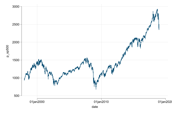
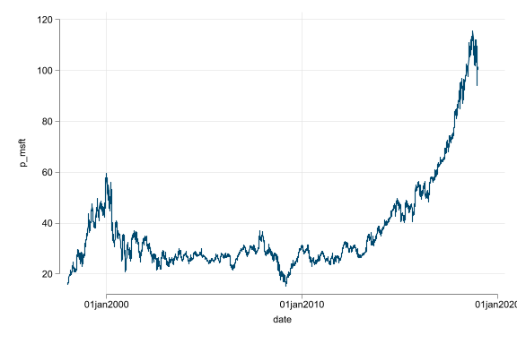
Microsoft and S&P 500 stock prices - data

  • Daily price of Microsoft stock and value of S&P 500 stock market index
  • The data covers 21 years starting with December 31 1997 and ending with December 31 2018.
  • Many decisions to make…
  • Look at data first

Case study: Stock price and stock market index value

Code
qui {
use "data_slides/stock-prices-daily.dta", clear
ren *, low
}
line p_sp500 date, name(m1, replace)
line p_msft date, name(m2, replace)

Time series comparisons - S&P 500 case study

Key decisions:

  • Daily price = closing price
  • Gaps will be overlooked
    • Friday-Monday gap ignored
    • Holidays (Christmas, 4 of July (when would be a weekday)
  • All values kept, extreme values part of process
  • In finance, portfolio managers often focus on monthly returns, Hence we choose monthly returns to analyze.
  • Take the last day of each month

Microsoft and S&P 500 stock prices - ts plot

Code
qui {
use "data_slides/stock-prices-daily.dta", clear
ren *, low
sort ym date
bysort ym: gen flag = _n == _N
keep if flag==1
}
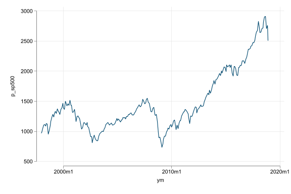
line p_sp500 ym, name(m1, replace)
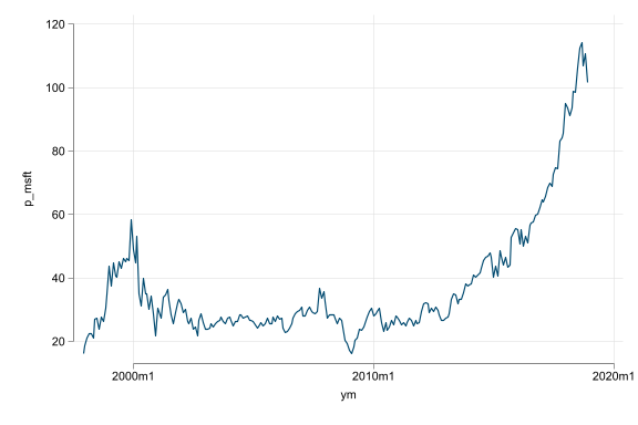
line p_msft ym, name(m2, replace)

Microsoft and S&P 500 stock prices - decisions 2

  • Monthly time series plot - easier to read
  • Additional decision needed: it is obviously non-stationary (Phillips-Perron test: very high p-value)
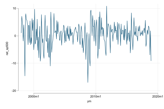
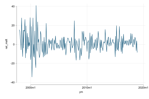
  • Use returns:
    • Returns: percent change of the closing prices: \(100\% \frac{y_t - y_{t-1}}{y_t}\).
    • monthly returns - take the closing price for the last day of a month
    • Alternative measure: first difference of log prices.

Microsoft and S&P 500 - index returns (pct)

Code
qui: {
use "data_slides/stock-prices-daily.dta", clear
ren *, low
sort ym date
bysort ym: gen flag = _n == _N
keep if flag==1
tsset ym
gen ret_sp500 = 100 * (p_sp500 - p_sp500[_n-1]) / p_sp500[_n-1]
gen ret_msft = 100 * (p_msft - p_msft[_n-1]) / p_msft[_n-1]
}

line ret_sp500 ym, name(m1, replace)
line ret_msft ym, name(m2, replace)

Unit root test: Microsoft and S&P 500 returns

Code
pperron ret_sp500
pperron ret_msft

Phillips–Perron test for unit root       Number of obs   = 251
Variable: ret_sp500                      Newey–West lags =   4

H0: Random walk without drift, d = 0

                                       Dickey–Fuller
                   Test      -------- critical value ---------
              statistic           1%           5%          10%
--------------------------------------------------------------
 Z(rho)        -230.845      -20.301      -14.000      -11.200
 Z(t)           -14.365       -3.460       -2.880       -2.570
--------------------------------------------------------------
MacKinnon approximate p-value for Z(t) = 0.0000.

Phillips–Perron test for unit root       Number of obs   = 251
Variable: ret_msft                       Newey–West lags =   4

H0: Random walk without drift, d = 0

                                       Dickey–Fuller
                   Test      -------- critical value ---------
              statistic           1%           5%          10%
--------------------------------------------------------------
 Z(rho)        -284.851      -20.301      -14.000      -11.200
 Z(t)           -19.346       -3.460       -2.880       -2.570
--------------------------------------------------------------
MacKinnon approximate p-value for Z(t) = 0.0000.

Regression with time series

Time series regressions: The same

  • Regression in time series data is defined and estimated the same way as in other data.

\[y^E_t = \beta_0 + \beta_1 x_{1t} + \beta_2 x_{2t} + \ldots\]

  • Interpretations similar to cross-section
    • \(\beta_0\): We expect \(y\) to be \(\beta_0\) when all explanatory variables are zero.
    • \(\beta_1\): Comparing time periods with different \(x_1\) but the same in terms of all other explanatory variables, we expect \(y\) to be higher by \(\beta_1\) when \(x_1\) is higher by one unit.

Time series regression: But different

  • With time series data, we often estimate regressions in changes
  • We use the \(\Delta\) notation for changes

\[\Delta x_t = x_t - x_{t-1}\]

  • The regression in changes is \[\Delta y^E_t = \alpha + \beta \Delta x_t\]

    • \(\alpha\): \(y\) is expected to change by \(\alpha\) when \(x\) doesn’t change
    • \(\beta\): \(y\) is expected to change by \(\beta\) more when \(x\) increases by one unit more

Time series regression: Growth

  • We often have variables in relative or percentage changes,

\[\%\Delta (y_t)^E = \alpha + \beta \%\Delta(x_t)\]

  • We can approximate relative differences by log differences, which are here log change: first taking logs of the variables and then taking the first difference

\[\Delta \ln(y_t) = \ln(y_t) - \ln(y_{t1})\]

Returns on a company stock and market returns

\[\%\Delta(\text{MSFT}_t) = \alpha + \beta \%\Delta (\text{SP500}_t)\]

  • \(\alpha = 0.54\); \(\beta = 1.26\)
  • Intercept: returns on the Microsoft stock tend to be 0.54 percent when the S%P500 index doesn’t change.
  • Slope: returns on the Microsoft stock tend to be 1.26% higher when the returns on the S&P500 index are 1% higher. The 95% CI is \([1.06, 1.46]\).
  • R-squared: 0.36
  • First difference of log prices. Estimate is 1.24
  • Daily returns (percent), beta is 1.10

Issues to deal with, before Regression: a laundry list

  • Handling trend(s) and random walk (RW)
    • Add trend variable or Difference the series
  • Transforming the series, such as taking first differences or percent change
  • Handling seasonality and special events
    • Include dummies
  • Reconsidering standard errors. Specially if series have Unit Roots
  • Dealing with serial correlation - taking time-to-build into account with lags

Trend & RW - Spurious regression

  • Trends, seasonality, and random walks can present serious threats to uncovering meaningful patterns in time series data.
    • Example: time series regression in levels \(y^E_t = \alpha + \beta x_t\).
    • If both \(y\) and \(x\) have a positive trend, the slope coefficient \(\beta\) will be positive whether the two variables are related or not.
    • Associations between variables only because of the effect of trends are said to be spurious correlation.
  • Think of trend and seasonality are confounders (omitted variables)
    • trend: global tendencies e.g. economic activity, fashion
    • seasonality: e.g. weather, holidays, human habits (sleep)
  • Another reason for spurious correlation is small sample size…

Trend & RW - solution: first differences

\[\Delta y^E_t = \alpha + \beta \Delta x_t\]

  • Coefficients have the same interpretation as before, but relate changes in variables.
  • Because variables denote changes…
    • \(\alpha\) is the average change in \(y\) when \(x\) doesn’t change.
    • The slope coefficient on \(\Delta x_t\) shows how much more \(y\) is expected to change when \(x\) changes by one more unit.
    • The slope shows how \(y\) is expected to change when \(x\) changes, in addition to \(\alpha\).

Seasonality in time series regressions

  • Capturing seasonality is also crucial.
  • Higher the frequency – the more important.
    • People behave differently on different hours and days
    • Weather varies over months
    • Holidays, ect
  • Have seasonal dummies if seasonality is stable.

\[y^E_t = \alpha + \beta x_t + \delta_{Jan} + \delta_{Feb} + \cdots + \delta_{Nov}\]

  • Pattern may vary over time. If it does, solutions must capture exact pattern – (difficult, not covering here)

Another Problem: Serial correlation

  • Serial correlation means correlation of a variable with its previous values

    • It usually refers to the correlation of the residuals with their previous values.
  • Order serial correlation coefficient is defined as \[\rho_k = \text{Corr}[x_t, x_{t-k}]\]

  • If independent variables are serially correlated, usually not a problem.

  • If dependent variable is serially correlated (the error), it is a problem.

  • Serial correlation makes the usual standard error estimates wrong.

    • Even classical heteroskedasticity robust SE is wrong - sometimes very wrong
  • More precisely it is serial correlation in residuals, but think about is as serial correlation in \(y_t\) is okay

Standard errors in time series regressions

  • In most time series, there will be some serial correlation

  • Sol1: Use the Newey-West SE: in Stata newey command.

    • This incorporates structure of serial correlation of the regression residuals
    • Fine if heteroskedasticity as well
    • Need to specify lags, based on frequency and seasonality
  • Sol2: Have lagged dependent variable in the regression (one lag is usually enough) \[y_t = \alpha + \beta x_t + \gamma_1 y_{t-1} + \gamma_2 y_{t-2} \ldots\]

    • This will change Coefficients and adjust SEs

Case study B: Electricity consumption and temperature

Electricity consumption and temperature

  • We have access to monthly weather and electricity data for Phoenix, Arizona: Overall 204 month
  • Also access to “cooling degree days” and “heating degree days” data
  • The cooling degree days measure Number of degrees that a day’s average temperature is above 65F (18C). This is add up over the month.
  • Similar for heating degree days but below 65F (18C)
  • Access to Electricity consumption data over the month
  • As expected, this values will be seasonal.

CS: Modelling decisions

  • There is an exponential trend in electricity –> use log difference
  • For easier interpretation, take first difference (FD) of cooling and heating days
  • Natural question: How much does electricity consumption change when temperature changes?
  • Add monthly dummies, January (December to January) is reference
  • Use Newey-West standard errors

Model estimates

Variables (1) (2)
\(\Delta\)CD 0.031** 0.017**
(0.001) (0.002)
\(\Delta\)HD 0.037** 0.014**
(0.003) (0.003)
month = 2, February -0.274**
month = 3, March -0.122**
Constant 0.001 0.092**
(0.002) (0.013)
Observations 203 203

Model results

  • Simple (1) model:
    • In months when cooling degrees increase by one degree and heating degrees do not change, electricity consumption increases by 3.1 percent, on average.
    • When heating degrees increase by one degree and cooling degrees do not change, electricity consumption increases by 3.7 percent, on average.
  • Model (2) with monthly dummies.
    • The reference month is January: constant (when cooling and heating degrees stay the same), electricity consumption increases by about 9% from December to January.
    • The other season coefficients compare to this change:
      • February: the January to February change is 28 percentage points lower than in the reference month, December to January.

Electricity consumption and temperature – different SE estimates

Variables (1) (2) (3)
Simple SE Newey–West SE Lagged dep.var
\(\Delta\)CD 0.017** 0.017** 0.017**
(0.002) (0.002) (0.002)
\(\Delta\)HD 0.014** 0.014** 0.014**
(0.002) (0.003) (0.002)
Lag of \(\Delta\) ln Q -0.002
(0.062)
Month dummies YES YES YES
Observations 203 203 202
R-squared 0.951 0.951
Standard errors in parentheses
** p<0.01, * p<0.05

Electricity consumption and temperature – different SE estimates

  • To correct for serial correlation, compare simple SE model with two correctly specified models
    • with Newey-West SE
    • with Lagged dependent variable
  • SE marginally different, and with lagged values, coefficients are also similar up to 3 digits
    • Similar, not the same
    • Sometimes substantial difference (if strong serial correlation)

Propagation effect

Propagation effect: changes and lags - FDL model

In time series, we can analyze how an impact builds up across several periods (time-to-build):

\[\Delta y^E_t = \alpha + \beta_0 \Delta x_t + \beta_1 \Delta x_{t-1} + \beta_2 \Delta x_{t-2}\]

  • \(\beta_0\) = how many units more \(y\) is expected to change within the same time period when \(x\) changes by one more unit (No change before or after).

  • \(\beta_1\) = how much more \(y\) is expected to change in the next time period after \(x\) changed by one more unit.

  • Cumulative effect: \(\beta_\text{cumul} = \beta_0 + \beta_1 + \beta_2\)

  • \(\beta_k\) are the short-term effects, \(\beta_\text{cumul}\) is the cumulative effect/Long Term Effect.

Testing the cumulative effect

  • To get a SE on the cumulative effect, do a trick and transformation, and estimate a different model

\[ \begin{aligned} \Delta y^E_t &= \alpha + \beta_0 \Delta x_t + \beta_1 \Delta x_{t-1} + \beta_2 \Delta x_{t-2} \\ \Delta y^E_t &= \alpha + (\beta_\text{cumul} - \beta_1 - \beta_2) \Delta x_t + \beta_1 \Delta x_{t-1} + \beta_2 \Delta x_{t-2} \\ \Delta y^E_t &= \alpha + \beta_\text{cumul} \Delta x_t + \beta_1 (\Delta x_{t-1}- \Delta x_t) + \beta_2 (\Delta x_{t-2} - \Delta x_t)\\ \Delta y^E_t &= \alpha + \beta_\text{cumul} \Delta x_{t} + \delta_0 \Delta(\Delta x_t) + \delta_1 \Delta(\Delta x_{t-1}) \end{aligned}\]

  • \(\beta_\text{cumul}\) is exactly the same as \(\beta_0 + \beta_1 + \beta_2\)
  • Usually estimate both. Separate and cumulative effect
  • Often need a few lags

Propagation effect: changes and lags - FDL model

See Case Study in Chapter 12

Summary of the process

  • Decide on frequency; deal with gaps if necessary.
  • Plot the series. Identify features and issues.
  • Handle trends by transforming variables (Often: first difference d.).
  • Specify regression that handles seasonality, usually by including season dummies.
  • Include or don’t include lags of the right-hand-side variable(s).
  • Handle serial correlation. newey or lagged dependent variable.
  • Interpret coefficients in a way that pays attention to potential trend and seasonality.
  • Time series econometrics very complicated beyond this.
  • But: These steps often good enough.

Main takeaways

  • Regressions with time series data allow for additional opportunities, but they pose additional challenges, too
  • Regressions with time series data help uncover associations from changes and associations across time
  • Trend, seasonality, and random walk-like non-stationarity are additional challenges
  • Do not regress variables that have trend or seasonality; without dealing with them they produce spurious results