Multiple Regression Analysis
When A5 Fails
Fernando Rios-Avila
What is Heteroskedasticity?
Mathematically: \[Var(e|x=c_1)\neq Var(e|x=c_2)\]
This means: the conditional variance of the errors is not constant across control characteristics.
Consequences
What happens when you have heteroskedastic errors?
In terms of \(\beta's\) and \(R^2\) and \(R^2_{adj}\), nothing. Coefficients and Goodness of fit are still unbiased and consistent.
But, Coefficients standard errors are based on the simplifying assumption of normality. Thus Variances will be bias!.
- If variances are biased, then all statistics will be wrong.
How bad can it be?
Setup:
\(y = e\) where \(e \sim N(0,\sigma_e^2h(x))\)
\(x = uniform(-1,1)\)
Code
/*capture program drop sim_het
program sim_het, eclass
    clear
    set obs 500
    gen x = runiform(-1,1)
    gen u = rnormal()
    ** Homoskedastic
    gen y_1 = u*2
    ** increasing first, decreasing later
    gen y_4 = u*sqrt(9*abs(x))
    replace x = x-2
    reg y_1 x
    matrix b=_b[x],_b[x]/_se[x]
    reg y_4 x
    matrix b=b,_b[x],_b[x]/_se[x]
    matrix coleq   b = h0 h0 h3 h3
    matrix colname b = b  t  b  t
    ereturn post b
end
qui:simulate , reps(1000) dots(100):sim_het
save mdata/simulate.dta, replace*/
use mdata/simulate.dta, replace
two (kdensity h0_b_t) (kdensity h3_b_t) ///
    (function y = normalden(x), range(-4 4) lw(2) color(gs5%50)), ///
    legend(order(3 "Normal" 1 "With Homoskedasticty" 2 "with Heteroskedasticity"))
graph export images/fig6_1.png, replace height(1000)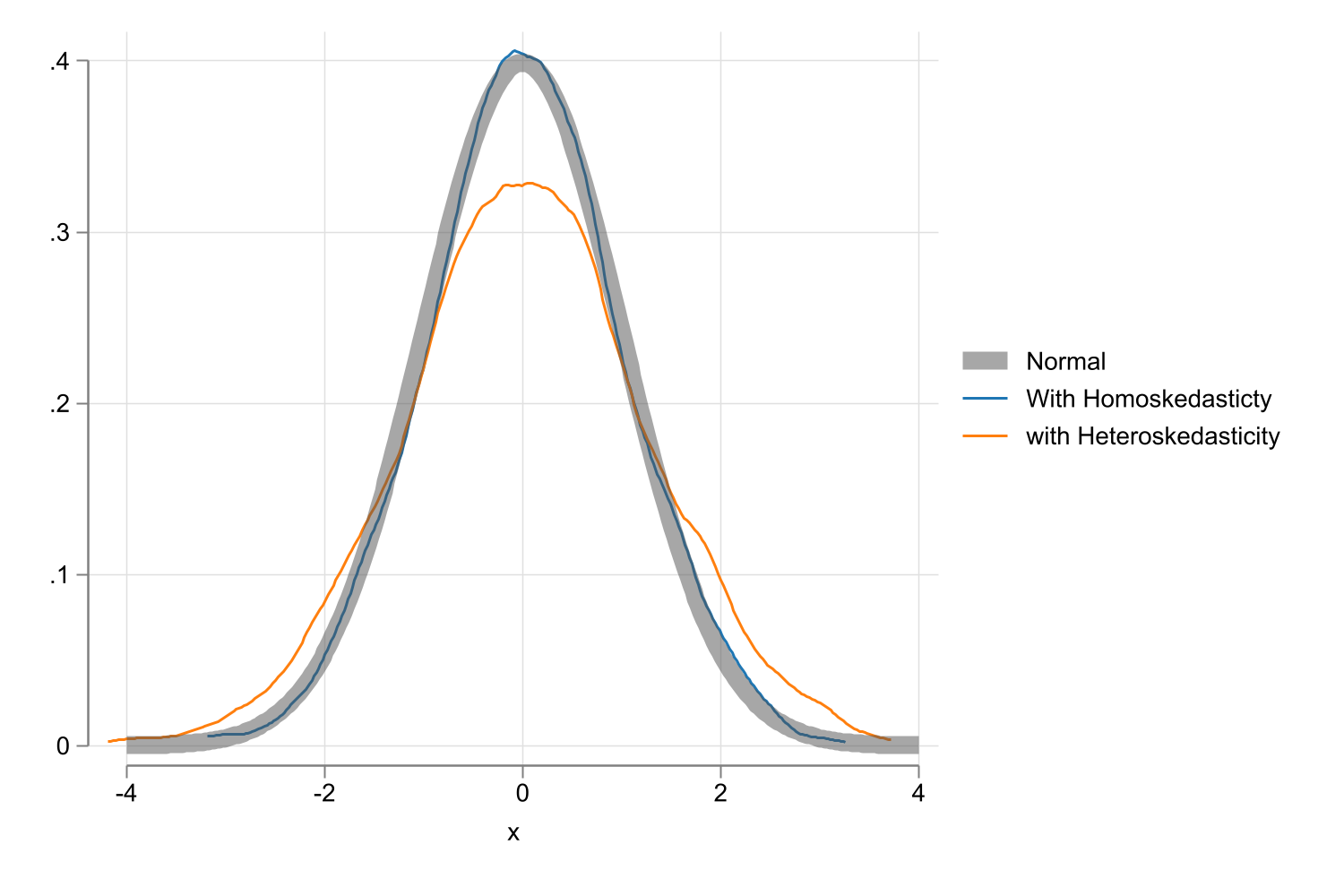
What to do about it?
What to do about it?
So, If errors are heteroskedastic, then all statistics (t-stats, F-stats, chi2’s) are wrong.
But, there are solutions…many solutions
- GLS: Generalized Least Squares
- WLS: Weighted Least Squares
- FGLS: Feasible Generealized Least Squares
- WFLS: Weighted FGLS
- HC0-HC3: Heteroskedasticity consistent SE
Some of them are more involved than others.
But before trying to do that, lets first ask…do we have a problem?
Detecting the Problem
- Consider the model:
\[y = \beta_0 + \beta_1 x_1 + \beta_2 x_2 +\beta_3 x_3 +e \]
- We usually start with the assumption that errors are homoskedastic \(Var(e|x's)=\sigma^2_c\).
- However, now we want to allow for the possibility of heteroskedasiticity. ie, that variance is some function of X.
- We have to test if the conditional variance is a function that varies with \(x\):
\[Var(e|x)=f(x_1,x_2,\dots,x_k) \sim a_0+a_1x_1 + a_2 x_2 + \dots + a_k x_k+v\]
\[Var(e|x)=f(x_1,x_2,\dots,x_k) \sim a_0+a_1x_1 + a_2 x_2 + \dots + a_k x_k+v\]
- This expression says the conditional variance can vary with \(X's\).
- It could be as flexible as needed, but linear is usually enough.
With this the Null hypothesis is: \[H_0: a_1 = a_2 = \dots = a_k=0 \text{ vs } H_1: H_0 \text{ is false} \]
Easy enough, but do we KNOW \(Var(e|x)\) ? can we model the equation?
We don’t!.
But we can use \(\hat e^2\) instead. The assumption is that \(\hat e^2\) is a good enough approximation for the condional variance \(Var(e|x)\).
With this, the test for heteroskedasticty can be implemented using the following recipe.
- Estimate \(y=x\beta+e\) and obtain predicted model errors \(\hat e\).
- Model \(\hat e^2 = \color{green}{h(x)}+v\), as a proxy for the variance model.
- \(h(x)\) could be estimated using some linear or nonlinear functional forms.
- Test if conditional variance changes with respect to any explanatory variables.
- The null is H0: Errors are Homoskedastic. Rejection the error suggests you have Heteroskedasticity.
- Note: Depending on Model specification, and test used, there are various Heteroskedasticity tests.
Heteroskedasticity tests:
\[\begin{aligned} \text{Model}: y &= \beta_0 + \beta_1 x_1 + \beta_2 x_2 + \beta_3 x_3 + e \\ \hat e & = y - (\hat \beta_0 + \hat\beta_1 x_1 +\hat \beta_2 x_2 +\hat \beta_3 x_3) \end{aligned} \]
Breusch-Pagan test:
\[\begin{aligned} \hat e^2 & = \gamma_0 + \gamma_1 x_1 +\gamma_2 x_2 +\gamma_3 x_3 + v \\ H_0 &: \gamma_1=\gamma_2=\gamma_3=0 \\ F &= \frac{R^2_{\hat e^2}/k}{(1-R^2_{\hat e^2})/(n-k-1)} \\ LM &=N R^2_{\hat e^2} \sim \chi^2(k) \leftarrow BP-test \end{aligned} \]
- Easy and simple, but only considers “linear” Heteroskedasticity
Heteroskedasticity tests:
\[\begin{aligned} \text{Model}: y &= \beta_0 + \beta_1 x_1 + \beta_2 x_2 + \beta_3 x_3 + e \\ \hat e & = y - (\hat \beta_0 + \hat\beta_1 x_1 +\hat \beta_2 x_2 +\hat \beta_3 x_3) \end{aligned} \]
White:
\[\begin{aligned} \hat e^2 & = \gamma_0 + \sum \gamma_{1,k} x_k + \sum \gamma_{2,k} x_k^2 + \sum_k \sum_{j\neq k} \gamma_{3,j,k} x_j x_k + v \\ H_0 &: \text{ All } \gamma's =0 \\ F &= \frac{R^2_{\hat e^2}/q}{(1-R^2_{\hat e^2})/(n-q-1)} \\ LM &=N R^2_{\hat e^2} \sim \chi^2(q) \end{aligned} \]
\(q\) is the total number of coefficients in the model (not counting the intercept.)
- Accounts for nonlinearities, but gets “messy” with more variables.
Heteroskedasticity tests:
\[\begin{aligned} \text{Model}: y &= \beta_0 + \beta_1 x_1 + \beta_2 x_2 + \beta_3 x_3 + e \\ \hat e & = y - (\hat \beta_0 + \hat\beta_1 x_1 +\hat \beta_2 x_2 +\hat \beta_3 x_3) \end{aligned} \]
Modified White:
\[\begin{aligned} \hat y &= y - \hat e \\ \hat e^2 & = \gamma_0 + \gamma_1 \hat y + \gamma_2 \hat y^2 + \dots + v \\ H_0 &: \gamma_1 = \gamma_2 = \dots =0 \\ F &= \frac{R^2_{\hat e^2}/ h }{(1-R^2_{\hat e^2})/(n-h-1)} \\ LM &=N R^2_{\hat e^2} \sim \chi^2(h) \end{aligned} \]
\(h\) is the total number of coefficients in the model (not counting the intercept.)
- Accounts for nonlinearities (because of how \(\hat y\) is constructed), and is simpler to implement.
- But, nonlinearity is restricted.
Example
Housing prices:
\[\begin{aligned} price &= \beta_0 + \beta_1 lotsize + \beta_2 sqft + \beta_3 bdrms + e_1 \\ log(price) &= \beta_0 + \beta_1 log(lotsize) + \beta_2 log(sqft) + \beta_3 bdrms + e_2 \\ \end{aligned} \]
frause hprice1, clear
reg price lotsize sqrft bdrms
predict res, res
predict price_hat
gen res2=res^2
display "BP-test"
reg res2  lotsize sqrft bdrms, notable
display "nR^2:   " e(N)*e(r2)
display "p(chi2) " %5.3f chi2tail(e(df_m),e(N)*e(r2))

display "White Test"
reg res2  c.(lotsize sqrft bdrms)##c.(lotsize sqrft bdrms), notable
display "nR^2:   " e(N)*e(r2)
display "p(chi2) " %5.3f chi2tail(e(df_m),e(N)*e(r2))

display "MWhite Test"
reg res2  price_hat c.price_hat#c.price_hat, notable
display "nR^2:   " e(N)*e(r2)
display "p(chi2) " %5.3f chi2tail(e(df_m),e(N)*e(r2))
      Source |       SS           df       MS      Number of obs   =        88
-------------+----------------------------------   F(3, 84)        =     57.46
       Model |  617130.701         3  205710.234   Prob > F        =    0.0000
    Residual |  300723.805        84   3580.0453   R-squared       =    0.6724
-------------+----------------------------------   Adj R-squared   =    0.6607
       Total |  917854.506        87  10550.0518   Root MSE        =    59.833

------------------------------------------------------------------------------
       price | Coefficient  Std. err.      t    P>|t|     [95% conf. interval]
-------------+----------------------------------------------------------------
     lotsize |   .0020677   .0006421     3.22   0.002     .0007908    .0033446
       sqrft |   .1227782   .0132374     9.28   0.000     .0964541    .1491022
       bdrms |   13.85252   9.010145     1.54   0.128    -4.065141    31.77018
       _cons |  -21.77031   29.47504    -0.74   0.462    -80.38466    36.84405
------------------------------------------------------------------------------
(option xb assumed; fitted values)
BP-test

      Source |       SS           df       MS      Number of obs   =        88
-------------+----------------------------------   F(3, 84)        =      5.34
       Model |   701213780         3   233737927   Prob > F        =    0.0020
    Residual |  3.6775e+09        84  43780003.5   R-squared       =    0.1601
-------------+----------------------------------   Adj R-squared   =    0.1301
       Total |  4.3787e+09        87  50330276.7   Root MSE        =    6616.6

nR^2: 14.092386
p(chi2) 0.003
White Test

      Source |       SS           df       MS      Number of obs   =        88
-------------+----------------------------------   F(9, 78)        =      5.39
       Model |  1.6784e+09         9   186492378   Prob > F        =    0.0000
    Residual |  2.7003e+09        78    34619265   R-squared       =    0.3833
-------------+----------------------------------   Adj R-squared   =    0.3122
       Total |  4.3787e+09        87  50330276.7   Root MSE        =    5883.8

nR^2: 33.731659
p(chi2) 0.000
MWhite Test

      Source |       SS           df       MS      Number of obs   =        88
-------------+----------------------------------   F(2, 85)        =      9.64
       Model |   809489395         2   404744697   Prob > F        =    0.0002
    Residual |  3.5692e+09        85  41991113.9   R-squared       =    0.1849
-------------+----------------------------------   Adj R-squared   =    0.1657
       Total |  4.3787e+09        87  50330276.7   Root MSE        =    6480.1

nR^2: 16.268416
p(chi2) 0.000
frause hprice1, clear
reg lprice llotsize lsqrft bdrms
predict res, res
predict price_hat
gen res2=res^2
display "BP-test"
reg res2 llotsize lsqrft bdrms, notable
display "nR^2: " e(N)*e(r2)
display "p(chi2) " %5.3f chi2tail(e(df_m),e(N)*e(r2))
display "White Test"
reg res2 c.(llotsize lsqrft bdrms)##c.(llotsize lsqrft bdrms), notable
display "nR^2: " e(N)*e(r2)
display "p(chi2) " %5.3f chi2tail(e(df_m),e(N)*e(r2))
display "MWhite Test"
reg res2 price_hat c.price_hat#c.price_hat, notable
display "nR^2: " e(N)*e(r2)
display "p(chi2) " %5.3f chi2tail(e(df_m),e(N)*e(r2))
      Source |       SS           df       MS      Number of obs   =        88
-------------+----------------------------------   F(3, 84)        =     50.42
       Model |  5.15504028         3  1.71834676   Prob > F        =    0.0000
    Residual |  2.86256324        84  .034078134   R-squared       =    0.6430
-------------+----------------------------------   Adj R-squared   =    0.6302
       Total |  8.01760352        87  .092156362   Root MSE        =     .1846

------------------------------------------------------------------------------
      lprice | Coefficient  Std. err.      t    P>|t|     [95% conf. interval]
-------------+----------------------------------------------------------------
    llotsize |   .1679667   .0382812     4.39   0.000     .0918404     .244093
      lsqrft |   .7002324   .0928652     7.54   0.000     .5155597    .8849051
       bdrms |   .0369584   .0275313     1.34   0.183    -.0177906    .0917074
       _cons |  -1.297042   .6512836    -1.99   0.050    -2.592191    -.001893
------------------------------------------------------------------------------
(option xb assumed; fitted values)
BP-test

      Source |       SS           df       MS      Number of obs   =        88
-------------+----------------------------------   F(3, 84)        =      1.41
       Model |  .022620168         3  .007540056   Prob > F        =    0.2451
    Residual |  .448717194        84  .005341871   R-squared       =    0.0480
-------------+----------------------------------   Adj R-squared   =    0.0140
       Total |  .471337362        87  .005417671   Root MSE        =    .07309

nR^2: 4.2232484
p(chi2) 0.238
White Test

      Source |       SS           df       MS      Number of obs   =        88
-------------+----------------------------------   F(9, 78)        =      1.05
       Model |  .051147864         9  .005683096   Prob > F        =    0.4053
    Residual |  .420189497        78  .005387045   R-squared       =    0.1085
-------------+----------------------------------   Adj R-squared   =    0.0057
       Total |  .471337362        87  .005417671   Root MSE        =     .0734

nR^2: 9.5494489
p(chi2) 0.388
MWhite Test

      Source |       SS           df       MS      Number of obs   =        88
-------------+----------------------------------   F(2, 85)        =      1.73
       Model |  .018464046         2  .009232023   Prob > F        =    0.1830
    Residual |  .452873315        85  .005327921   R-squared       =    0.0392
-------------+----------------------------------   Adj R-squared   =    0.0166
       Total |  .471337362        87  .005417671   Root MSE        =    .07299

nR^2: 3.4472889
p(chi2) 0.178
Can you do this in Stata? Yes, estat hettest. But look into the options. There are many more options in that command.
What do you do when you have Heteroskedasticity?
We need to fix!
- Recall, the problem is that \(Var(e|X)\neq c\)
- This affects how standard errors are estimated (we required homoskedasticity). But what happens when Homoskedasticity doesnt hold?
- We can “fix/change” the model, so its no longer heteroskedastic, and Standard Inference works. (FGLS, WLS)
- We neec to account for heteroskedasticity when estimating the variance covariance model.
So lets learn to Fix it first
How do we Fix Heteroskedasticity?
- In order to address the problem of heteroskedasticity, we require knowledge of why the model is heteroskedastic, or what is generating it.
\[Var(e|X)=h(x)\sigma^2_e \]
- Where \(h(x)\) is the “source” of heteroskedasticity, which may be a known or estimated function of \(x\).
- Which should be an strictly possitive function of \(x's\).
Knowledge is power
- If you know \(h(x)\), correcting heteroskedasticity is “easy”. Consider the following:
\[\begin{aligned} y &= b_0 + b_1 x_1 + b_2 x_2 + b_3 x_3 +e \\ Var(e|x) &=x_1 \sigma_e^2 || h(x)=x_1 \end{aligned} \]
You can correct Heteroskedasticity in two ways:
- Transform model by dividing everything by \(\sqrt{h(x)}\): \[\begin{aligned} \frac{y}{\sqrt{x_1}} &= b_0 \frac{1}{\sqrt{x_1}}+ b_1 \sqrt{x_1} + b_2 \frac{x_2}{\sqrt{x_1}} + b_3 \frac{x_3}{\sqrt{x_1}} +\frac{e}{\sqrt{x_1}} \\ Var\left(\frac{e}{\sqrt{x_1}}|x\right) &= \frac{1}{x_1} x_1\sigma_e^2=\sigma_e^2 \end{aligned} \]
The new error is Homoskedastic (but has no constant)!
- Estimate the model using by \(\frac{1}{h(x)}\) as weights: \[\begin{aligned} \beta=\min_\beta \sum \frac{1}{h(x)} (y-(b_0 + b_1 x_1 + b_2 x_2 + b_3 x_3))^2 \end{aligned} \]
Same solution as before, and there is no need to “transform” data, or keep track of a constant.
This is often called WLS (weighted least squares) or GLS (Generalized Least Squares).
- Interestingly: These approaches are more efficient than Standard OLS.
- Uses more information (heteroskedasticity)
- Makes better use of information (More weight to better data) Standard errors are smaller.
- t-stats, F-stats, etc now are valid.
- Coefficients will NOT be the same as before.
- \(R^2\) is less useful
- Heteroskedasticty test on transformed data may required added work.
FGLS: We do not know \(h(x)\), but we can guess
- If \(h(x)\) is not known, we can use an auxiliary model to estimate it:
\[\begin{aligned} Var(e|x) &= \sigma^2 \exp(\delta_0 + \delta_1 x_1 + \delta_2 x_2 +\dots) \exp v \\ \hat e^2 &= \sigma^2 \exp(\delta_0 + \delta_1 x_1 + \delta_2 x_2 +\dots) \exp v \\ log(\hat e^2) &= \delta_0 + \delta_1 x_1 + \delta_2 x_2 +\dots+ v \\ log(\hat e^2) &= \delta_0 + \delta_1 \hat y + \delta_2 \hat y^2 + \dots+ v \\ \widehat{\log h(x)} &= \hat \delta_0 + \hat \delta_1 x_1 + \hat \delta_2 x_2 + \dots = x \hat \delta \\ \hat h(x) &= \exp (x \hat \delta) \text{ or } \hat h(x)=e^{x \hat \delta} \end{aligned} \]
- Proceed as before (weighted or transformed)
- Its call Feasible GLS, because we need to estimate \(h(x)\).
Do not Correct, account for it: GLS and FGLS
Recall “Long” variance formula:
\[Var(\beta)=\color{brown}{(X'X)^{-1}}\color{green}{X}'\color{red}{Var(e|X)}\color{green}{X}\color{brown}{(X'X)^{-1}} \]
- The red part is a \(N\times N\) VCOV matrix of ALL erros. It can be Simplified with what we know!
\[\begin{aligned} Var_{gls/fgls}(\beta)&=\sigma^2_{\tilde e} \color{brown}{(X'X)^{-1}}\color{green}{X}'\color{red}{ \Omega_h(x) }\color{green}{X}\color{brown}{(X'X)^{-1}} \\ \sigma^2_{\tilde e} &= \frac{1}{N-k-1} \sum \frac{\hat e^2}{h(x)} \\ \Omega_h(x) [i,j] &= h(x_i) & \text{ if } i=j \\ & = 0 & \text{ if } i\neq j \\ \end{aligned} \]
- SE are corrected, but coefficients remain the same!
Do not Correct, account for it: White Sandwich Formula
- What if we do not want to even try guessing \(h(x)\)?
- you can use Robust Standard errors!
- Heteroskedastic Consistent SE to Heterosedasticity of unknown form.
Let me present to you, the Sandwitch Formula: \[Var(\beta)=c \color{brown}{(X'X)^{-1}}\color{green}{X}'\color{red}{\Omega}\color{green}{X}\color{brown}{(X'X)^{-1}} \]
\[\begin{aligned} \Omega [i,j] &= \hat e_i^2 & \text{ if } i=j \\ & = 0 & \text{ if } i\neq j \\ \end{aligned} \]
The best approximation to conditional variance is equal to \(\hat e_i^2\). (plus assuming no correlation)
Valid in large samples, but can be really bad in smaller ones.
There are other versions. See HC0 HC1 HC2 HC3.
What if did \(h(x)\), and it was wrong
- Using FGLS will change coefficients a bit. If they change a lot, It could indicate other assumptions in the model are incorrect. (functional form or exogeneity)
- In either case, you could always combine FGLS with Robust Standard Errors!
Statistical Inference
- If applying GLS or FGLS via transformations or reweighting. All we did before is valid.
- If using Robust standard errors (HC), t-stats are constructed as usual, but
- F-stats formulas are no longer valid.
Instead…use the long formula
\[\begin{aligned} H_0: & R_{q,k+1}\beta_{k+1,1}=c_{q,1} \\ \Sigma_R &= R_{q,k+1} V^r_\beta R'_{q,k+1} \\ F-stat &= \frac 1 q (R\beta-c)' \Sigma_R^{-1} (R\beta-c) \end{aligned} \]
Extra: Prediction and SE
Prediction SE:
- If you are using GLS, Formulas seen before apply with the following modification: \(Var(e|X=x_0)=\sigma^2_{\tilde e} h(x_0)\)
- If you are using FGLS, its not that simple because of the two-step modeling
For Prediction with Logs
- You need to take into account Heteroskedasticity
\[\hat y_i = \exp \left( \widehat{log y_i}+\hat \sigma_{\tilde e}^2 \hat h_i /2 \right) \]
Example
frause smoke, clear
gen age_40sq=(age-40)^2
** Default
qui:reg cigs lincome lcigpric educ age age_40sq restaurn
est sto m1
predict cig_hat
predict cig_res,res
** GLS: h(x)=lincome Weighted
qui:reg cigs lincome lcigpric educ age age_40sq restaurn [aw=1/lincome]
est sto m2
** FGLS: h(x) = f(cigs_hat)
gen lcres=log(cig_res^2)
qui:reg lcres c.cig_hat##c.cig_hat##c.cig_hat
predict aux
gen hx=exp(aux)
qui:reg cigs lincome lcigpric educ age age_40sq restaurn [aw=1/hx]
est sto m3
qui:reg cigs lincome lcigpric educ age age_40sq restaurn , robust
est sto m4
qui:reg cigs lincome lcigpric educ age age_40sq restaurn [aw=1/lincome], robust
est sto m5
qui:reg cigs lincome lcigpric educ age age_40sq restaurn [aw=1/hx], robust
est sto m6
set linesize 255
Code
------------------------------------------------------------------------------------------------------------
                  default             GLS            FGLS             Rob         GLS-Rob        FGLS-Rob
                   b/se/p          b/se/p          b/se/p          b/se/p          b/se/p          b/se/p
------------------------------------------------------------------------------------------------------------
lincome             0.880           0.926           1.005**         0.880           0.926*          1.005
                  (0.728)         (0.672)         (0.422)         (0.596)         (0.559)         (0.651)
                  [0.227]         [0.169]         [0.017]         [0.140]         [0.098]         [0.123]

lcigpric           -0.751          -1.525          -4.572          -0.751          -1.525          -4.572
                  (5.773)         (5.696)         (4.260)         (6.035)         (6.067)         (9.651)
                  [0.897]         [0.789]         [0.284]         [0.901]         [0.802]         [0.636]

educ               -0.501***       -0.477***       -0.610***       -0.501***       -0.477***       -0.610***
                  (0.167)         (0.166)         (0.115)         (0.162)         (0.159)         (0.115)
                  [0.003]         [0.004]         [0.000]         [0.002]         [0.003]         [0.000]

age                 0.049           0.048           0.041           0.049*          0.048           0.041
                  (0.034)         (0.033)         (0.026)         (0.030)         (0.029)         (0.032)
                  [0.146]         [0.147]         [0.108]         [0.099]         [0.101]         [0.197]

age_40sq           -0.009***       -0.009***       -0.007***       -0.009***       -0.009***       -0.007***
                  (0.002)         (0.002)         (0.001)         (0.001)         (0.001)         (0.002)
                  [0.000]         [0.000]         [0.000]         [0.000]         [0.000]         [0.001]

restaurn           -2.825**        -2.776**        -3.383***       -2.825***       -2.776***       -3.383***
                  (1.112)         (1.108)         (0.722)         (1.008)         (0.992)         (0.696)
                  [0.011]         [0.012]         [0.000]         [0.005]         [0.005]         [0.000]

_cons              10.797          13.184          25.712          10.797          13.184          25.712
                 (24.145)        (23.656)        (17.120)        (25.401)        (25.478)        (41.539)
                  [0.655]         [0.577]         [0.134]         [0.671]         [0.605]         [0.536]
------------------------------------------------------------------------------------------------------------
N                     807             807             807             807             807             807
------------------------------------------------------------------------------------------------------------
LPM revised
- What was wrong with LPM?
- Fixed marginal effects (depends on functional form)
- May predict p>1 or p<0
- It is Heteroskedastic by construction
- But now we know how to deal with this! GLS (why not FGLS) and Robust
- In LPM: \(Var(y|x)=p(x)(1-p(x)) = \hat y (1-\hat y)\)
- We can use this to transform or weight the data!
- Only works if \(0<p(x)<1\).
LPM Example
frause gpa1, clear
** LPM
gen parcoll = (fathcoll | mothcoll)
reg pc hsgpa act parcoll
predict res_1, res
      Source |       SS           df       MS      Number of obs   =       141
-------------+----------------------------------   F(3, 137)       =      1.98
       Model |  1.40186813         3  .467289377   Prob > F        =    0.1201
    Residual |  32.3569971       137  .236182461   R-squared       =    0.0415
-------------+----------------------------------   Adj R-squared   =    0.0205
       Total |  33.7588652       140  .241134752   Root MSE        =    .48599

------------------------------------------------------------------------------
          pc | Coefficient  Std. err.      t    P>|t|     [95% conf. interval]
-------------+----------------------------------------------------------------
       hsgpa |   .0653943   .1372576     0.48   0.635    -.2060231    .3368118
         act |   .0005645   .0154967     0.04   0.971    -.0300792    .0312082
     parcoll |   .2210541    .092957     2.38   0.019      .037238    .4048702
       _cons |  -.0004322   .4905358    -0.00   0.999     -.970433    .9695686
------------------------------------------------------------------------------(option xb assumed; fitted values)
Variable | Obs Mean Std. dev. Min Max
-------------+---------------------------------------------------------
pchat | 141 .3971631 .1000667 .1700624 .4974409
hx | 141 .2294822 .0309768 .1411412 .2499934(analytic weights assumed)
(sum of wgt is 628.1830743667746)
Source | SS df MS Number of obs = 141
-------------+---------------------------------- F(3, 137) = 2.22
Model | 1.54663033 3 .515543445 Prob > F = 0.0882
Residual | 31.7573194 137 .231805251 R-squared = 0.0464
-------------+---------------------------------- Adj R-squared = 0.0256
Total | 33.3039497 140 .237885355 Root MSE = .48146
------------------------------------------------------------------------------
pc | Coefficient Std. err. t P>|t| [95% conf. interval]
-------------+----------------------------------------------------------------
hsgpa | .0327029 .1298817 0.25 0.802 -.2241292 .289535
act | .004272 .0154527 0.28 0.783 -.0262847 .0348286
parcoll | .2151862 .0862918 2.49 0.014 .04455 .3858224
_cons | .0262099 .4766498 0.05 0.956 -.9163323 .9687521
------------------------------------------------------------------------------** Testing for Heteroskedasticity
replace res_1 = res_1^2
replace res_2 = res_2^2/hx
display "Default"
reg res_1 hsgpa act parcoll, notable
display "Weighted"
reg res_2 hsgpa act parcoll, notable(141 real changes made)
(141 real changes made)
Default
Source | SS df MS Number of obs = 141
-------------+---------------------------------- F(3, 137) = 2.82
Model | .133163365 3 .044387788 Prob > F = 0.0412
Residual | 2.15497574 137 .01572975 R-squared = 0.0582
-------------+---------------------------------- Adj R-squared = 0.0376
Total | 2.28813911 140 .016343851 Root MSE = .12542
Weighted
Source | SS df MS Number of obs = 141
-------------+---------------------------------- F(3, 137) = 0.63
Model | .874194807 3 .291398269 Prob > F = 0.5980
Residual | 63.5472068 137 .463848225 R-squared = 0.0136
-------------+---------------------------------- Adj R-squared = -0.0080
Total | 64.4214016 140 .460152868 Root MSE = .68106
The end…for now
Next Week: Problems of Specification