Limited Dependent Variable Models

MLE-Mua ha ha ha

Fernando Rios-Avila

What do we mean Limited??

Code
clear
set obs 2000
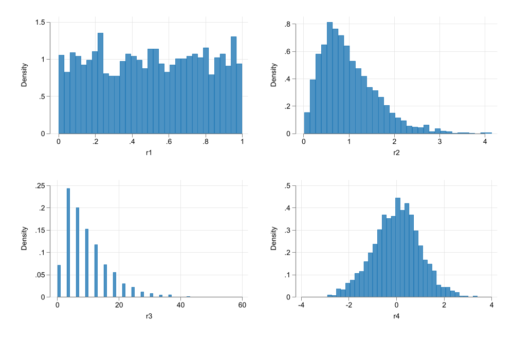
gen r1 = runiform()
gen r2 = rchi2(5)/5 
gen r3 = round(rchi2(3))*3
gen r4 = rnormal()
set scheme white2
color_style tableau
histogram r1, name(m1, replace) 
histogram r2, name(m2, replace)
histogram r3, name(m3, replace) width(1)  
histogram r4, name(m4, replace)
graph combine m1 m2 m3 m4
graph export images/fig9_1.png, width(1000) replace

Limited Dependent variables

What do we mean Limited??

  • When we think about “limited dependent variable” models, we refer to models when the distribution of the dep.variable is “limited”
    • In other words. The values it can take are restricted! (positive, or only integer), within a range, etc
  • Can you still use LRM for them?
  • Will anything change if you do?
  • Do we care?

No we dont, but..

  • We dont really care. In fact we have already use LRM on that fashion:
    • LPM: Dep variable was a Dummy
    • Wages: Always positive
    • # Children: Countable
  • But, there are couple of things one should consider.
    1. Models of this kind are usually heteroskedastic by construction. (robust? Weighted?)
    2. Predictions could made no sense.
    3. There are better models we could use to analyze the data

Better under some assumptions

  • However, this models cannot be estimated using OLS (there is no “close form solution”)
  • We may need to learn a new method: Maximum Likelihood

Probits and Logits

  • LPM are easy, fast, and good for most data analysis (exploration). But they have some limitations.
  • Most limitations can be overcome with alternative models: Logit or Probit
  • In constrast with LPM (which aims to explain individual outcomes), Logit/probit aims to explain Conditional Probabilities:

\[p(y=1|x) = G(x\beta)\]

  • where the function \(G()\) makes sure the predicted outcome is always between 0 and 1.
  • Caveat: Because \(G()\) is nonlinear, this is a nonlinear model, and marginal effects are harder to estimate.

What to use for \(G()\)

  • Two leading options:

\[logit: G(x\beta) = \frac{\exp{x\beta}}{1+\exp{x\beta}}\] \[probit: G(x\beta) = \Phi(x\beta)=\int_{-\infty}^{x\beta}\phi(z)dz\]

  • But in practice Either will work. Then why the difference?

Probits and Logits: Latent variables

  • It all comes down to the Latent variable!

  • Assumption:

    • Everybody has a latent score on every “binary” decision: The value to a decision \(y^*\) \[y^* = x\beta + e \]

    • If \(y^*\) is above certain threshold (\(y^*>0\)), you “do” something (\(y=1\)). If not you dont (\(y=0\)).

  • Thus the choice between logit and probit depends on the distribution of \(e\).

    • \(e\) is normal, then probit
    • \(e\) is logistic, then logit

Some Math

Latent Model:

\[ y^* = x\beta + e \]

We aim to measure the probablity of a positive latent.

\[\begin{aligned} P(y^*>0|x) & = P(x\beta + e>0|x) \\ & = P( e>- x\beta|x) \\ & = 1 - P( e < - x\beta|x) = 1-G( - x\beta|x) \\ & = G(x\beta) \end{aligned} \]

last step valid only if \(G()\) is symetrical.

Marginal Effects?

  • Same as before. The partial derivative!

\[\begin{aligned} p(y=1|x) &= G(\beta_0 + \beta_1 x_1 +\beta_2 x_2 ) \\ \frac{\partial p(y=1|x)}{\partial x_1} = G'(x\beta)\beta_1=g(x\beta)\beta_1 \end{aligned} \]

  • But if variables are dummies, we need to estimate true effect.

\[\begin{aligned} p(y=1|x) &= G(\beta_0 + \beta_1 x_1 +\beta_2 D_2 ) \\ \frac{\partial p(y=1|x)}{\partial D_2} = G(\beta_0 + \beta_1 x_1 +\beta_2 )-G(\beta_0 + \beta_1 x_1 ) \end{aligned} \]

and yes, you could also have interactions, polynomials, etc

MLE: How does this work?

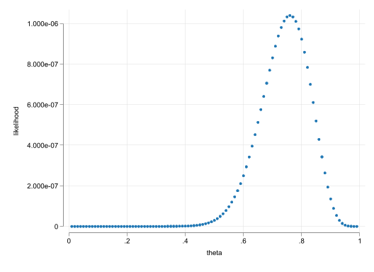
  • MLE: Maximum Likelihood Estimator, is an alternative method to OLS that allows you to estimate parameters in nonlinear models.

  • The idea of the method is to “model” the conditional distribution of the data \(F(y|x,\theta)\) or \(f(y|x,\theta)\), assuming \(X's\) are given and modifying values of \(\theta\) (distribution parameters).

  • \(LRM\) could be estimated via MLE, but you will need More assumptions:

    • The error \(e\) is normal.
  • Then “simply” find the parameters for the mean and variance that “maximizes” the probability that data Comes a given distribution.

  • In the case of Probit/logit, there is “only” one paramter we need to identify. The conditional probabilty \(p(y=1|X)\).

    • Except that we allow this to vary by \(X\)

Likelihood function for Logit/probit

\[L_i = G(x\beta)^{y=1}*(1-G(x\beta))^{y=0} \]

Under Independence:

\[L_D = L_1 \times L_2 \times \dots L_N \]

Thus we need to find the \(\beta's\) that make \(L_D\) the largest.

But because we like sums over products:

\[LL_D = \sum_{i=1}^N log(L_i) \]

Code
  clear
  set obs 25
  gen r = runiform()<.7
  mata: 
    r = st_data(.,"r")
    ll = J(99,2,0)
    for(i=1;i<=99;i++){
      theta = i/100
      // Log Properties
      ll[i,]= theta,exp(sum(log(theta:^(r:==1) :* (1-theta):^(r:==0))))
    }
  end
  qui getmata ll*=ll , force
  ren ll1 theta
  ren ll2 likelihood
  *scatter likelihood theta 
Number of observations (_N) was 0, now 25.

Testing?

  • You can test two things:

    • Test coefficients (\(\beta\))
    • Test marginal effects (\(G'(x\beta)\beta\))
  • Both test will most likely agree with each other, but some contradictions may arise. ### How?

  • z-test and/or Wald test: Similar to t-test and Joint F-test we cover before. But, we now make the assumption of normality (not t-distribution)

  • Log-Likelihood test. Similar to F-test for restricted and unrestricted model:

    • Estimate both Restricted and unrestricted model. And obtain their Log Likelihoods (\(\mathcal{L}_ur\)) and (\(\mathcal{L}_r\)).

    \[LR = 2 (\mathcal{L}_ur-\mathcal{L}_r) \overset{a}\sim \chi^2_q\]

Stata - Example

Code
frause mroz, clear
* LPM with Robust Standard errors
qui:reg inlf nwifeinc educ exper expersq age kidslt6 kidsge6, robust
est sto m1
qui:logit inlf nwifeinc educ exper expersq age kidslt6 kidsge6, 
est sto m2a
qui:margins, dydx(*) post
est sto m2b
probit inlf nwifeinc educ exper expersq age kidslt6 kidsge6, 
est sto m3a
qui:margins, dydx(*) post
est sto m3b

Iteration 0:   log likelihood =  -514.8732  
Iteration 1:   log likelihood = -402.06651  
Iteration 2:   log likelihood = -401.30273  
Iteration 3:   log likelihood = -401.30219  
Iteration 4:   log likelihood = -401.30219  

Probit regression                                       Number of obs =    753
                                                        LR chi2(7)    = 227.14
                                                        Prob > chi2   = 0.0000
Log likelihood = -401.30219                             Pseudo R2     = 0.2206

------------------------------------------------------------------------------
        inlf | Coefficient  Std. err.      z    P>|z|     [95% conf. interval]
-------------+----------------------------------------------------------------
    nwifeinc |  -.0120237   .0048398    -2.48   0.013    -.0215096   -.0025378
        educ |   .1309047   .0252542     5.18   0.000     .0814074     .180402
       exper |   .1233476   .0187164     6.59   0.000     .0866641    .1600311
     expersq |  -.0018871      .0006    -3.15   0.002     -.003063   -.0007111
         age |  -.0528527   .0084772    -6.23   0.000    -.0694678   -.0362376
     kidslt6 |  -.8683285   .1185223    -7.33   0.000    -1.100628    -.636029
     kidsge6 |    .036005   .0434768     0.83   0.408     -.049208    .1212179
       _cons |   .2700768    .508593     0.53   0.595    -.7267473    1.266901
------------------------------------------------------------------------------
Code
set linesize 255
*| classes: larger
display "Prob Models"
esttab m1 m2a m2b m3a m3b, scalar(r2 ll) cell(b(fmt(%5.3f)) ///
se(par([ ])) p( par(( )) ) )  gap  mtitle(LPM Logit Logit-mfx Probit Probit-mfx)
Prob Models

-----------------------------------------------------------------------------
                      (1)          (2)          (3)          (4)          (5)
                      LPM        Logit    Logit-mfx       Probit   Probit-mfx
                   b/se/p       b/se/p       b/se/p       b/se/p       b/se/p
-----------------------------------------------------------------------------
main                                                                         
nwifeinc           -0.003       -0.021       -0.004       -0.012       -0.004
                  [0.002]      [0.008]      [0.001]      [0.005]      [0.001]
                  (0.026)      (0.011)      (0.010)      (0.013)      (0.012)

educ                0.038        0.221        0.039        0.131        0.039
                  [0.007]      [0.043]      [0.007]      [0.025]      [0.007]
                  (0.000)      (0.000)      (0.000)      (0.000)      (0.000)

exper               0.039        0.206        0.037        0.123        0.037
                  [0.006]      [0.032]      [0.005]      [0.019]      [0.005]
                  (0.000)      (0.000)      (0.000)      (0.000)      (0.000)

expersq            -0.001       -0.003       -0.001       -0.002       -0.001
                  [0.000]      [0.001]      [0.000]      [0.001]      [0.000]
                  (0.002)      (0.002)      (0.001)      (0.002)      (0.001)

age                -0.016       -0.088       -0.016       -0.053       -0.016
                  [0.002]      [0.015]      [0.002]      [0.008]      [0.002]
                  (0.000)      (0.000)      (0.000)      (0.000)      (0.000)

kidslt6            -0.262       -1.443       -0.258       -0.868       -0.261
                  [0.032]      [0.204]      [0.032]      [0.119]      [0.032]
                  (0.000)      (0.000)      (0.000)      (0.000)      (0.000)

kidsge6             0.013        0.060        0.011        0.036        0.011
                  [0.014]      [0.075]      [0.013]      [0.043]      [0.013]
                  (0.337)      (0.422)      (0.421)      (0.408)      (0.407)

_cons               0.586        0.425                     0.270             
                  [0.152]      [0.860]                   [0.509]             
                  (0.000)      (0.621)                   (0.595)             
-----------------------------------------------------------------------------
N                     753          753          753          753          753
r2                  0.264                                                    
ll                 -423.9       -401.8                    -401.3             
-----------------------------------------------------------------------------
display "LR test"
qui:probit inlf nwifeinc educ exper expersq age kidslt6 kidsge6 motheduc fatheduc, 
est sto unrestricted
qui:probit inlf nwifeinc educ exper expersq age kidslt6 kidsge6 , 
est sto restricted
lrtest unrestricted restricted
LR test

Likelihood-ratio test
Assumption: restricted nested within unrestricted

 LR chi2(2) =   0.29
Prob > chi2 = 0.8668

Break? (5 mins!)

Censored and Truncated Data

  • Logits and Probits, are not the only models that require MLE for estimation.
    • Among Discrete data models, you also have ologit/oprobit for ordered responses. mlogit/mprobit for unordered ones. Extends on logit/probit.
  • There are other interesting cases:
    • When Data is censored.
    • When Data is truncated.

Three Cases

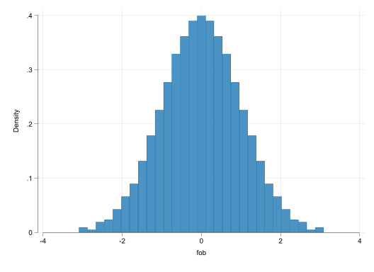
  • \(y\) is “conditionally-normal” and is Fully Observed.
  • You can estimate the model using OLS or ML
Code
qui:{
  clear
  set obs 999
  gen p   = _n/(_N+1)
  gen fob = invnormal(p)
}
qui:histogram fob

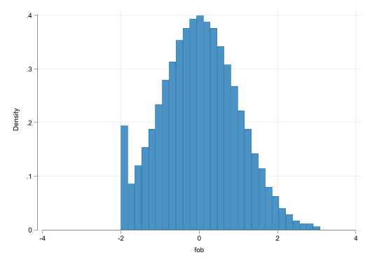
  • Data is observed for everyone, but is “censored” for some. tobit
    • Either corner solution (how many hours you study) or Recoded: \(y_{obs} = max(c,y^*)\)
Code
qui: replace fob = -2 if fob<-2
qui:histogram fob, xlabel(-4 (2) 4)

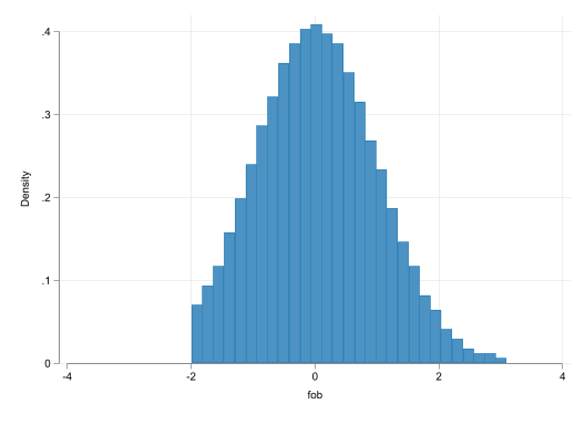
  • Below (or above) some threshold, you do not have information on \(y\). truncreg \[y_{obs} = y^* \text{ if } y^*>c\]

Estimation: Censored and Corner Solution

If data is censored or corner solution the estimation strategy is based on:

\[\begin{aligned} L_i &= \frac{1}{\sigma} \phi\left( \frac{y-x\beta}{\sigma} \right) \text{ if } y>c \\ &= 1-\Phi\left(\frac{x\beta}{\sigma} \right) \text{ if } y\leq c \\ \end{aligned} \]

If data is truncated, we need to “adjust” the distribution of what is observed

\[\begin{aligned} L_i &= \frac{1}{\Phi\left( x\beta/\sigma \right)} \frac{1}{\sigma} \phi\left( \frac{y-x\beta}{\sigma} \right) \text{ if } y>c \\ \end{aligned} \]

We will put -truncated regression- on the side for now. But see here for an example.

Interpretation: It depends!

  • What are you interested in analyzing? and what type of data you have?
  • Easiest Case. Just need to consider the coefficients (as in LRM)

\[ \begin{aligned} E(y^*|x) &= x\beta \\ \frac{\partial E(y^*|x)}{\partial x } &= \beta_x \end{aligned} \]

  • The same applies if model was censored.
  • Its an alternative approach to Probit models, where you are interest in analyzing why is data Not censored, or why is it above some threshold. (why people work)

  • Extensive margin effect. \[ \begin{aligned} P(y>0|x) &= \Phi\left(\frac{x\beta}{\sigma}\right) \\ \frac{\partial P(y>0|x)}{\partial x } &= \frac{\beta_x}{\sigma} \phi\left(\frac{x\beta}{\sigma}\right) \end{aligned} \]

Note: Coefficients \(\beta\) need to be Standardized.

  • If corner solution, one may be interested in the effect of those with positive outcomes only.

  • This is the intensive margin effect. \[ \begin{aligned} E(y|y>0,x) &= x\beta + \sigma \frac{\phi(x\beta / \sigma )}{\Phi(x\beta / \sigma )} \\ \frac{\partial E(y|y>0,x)}{\partial x } &= \beta_x \left[ 1-\frac{\phi(x\beta / \sigma )}{\Phi(x\beta / \sigma )} \left( \frac{x\beta }{\sigma }+ \frac{\phi(x\beta / \sigma )}{\Phi(x\beta / \sigma )}\right) \right] \end{aligned} \]

  • In this case, one may be interested in estimating the expected effect on everyone.
  • Combines both Intensive and extensive margin effects. Comparable to OLS.

\[ \begin{aligned} E(y|x) &= p(y>0|x)*E(y|y>0,x) + (1-p(y>0|x))*0 \\ \frac{\partial E(y|x)}{\partial x } &= \beta_x \Phi(x\beta) \end{aligned} \]
Example

Code
frause mroz, clear
qui:tobit hours nwifeinc educ c.exper##c.exper   age kidslt6 kidsge6 , ll(0)
qui:emargins, dydx(*) estore(m1)
qui:emargins, dydx(*) predict(p(0,.)) estore(m2)
qui:emargins, dydx(*) predict(e(0,.)) estore(m3)
qui:emargins, dydx(*) predict(ystar(0,.)) estore(m4)
esttab m1 m2 m3 m4, mtitle(Latent P(y>0) E(y|y>0) E(y) ) b(3) se

----------------------------------------------------------------------------
                      (1)             (2)             (3)             (4)   
                   Latent          P(y>0)        E(y|y>0)            E(y)   
----------------------------------------------------------------------------
nwifeinc           -8.814*         -0.002*         -3.969*         -5.189*  
                  (4.459)         (0.001)         (2.008)         (2.621)   

educ               80.645***        0.022***       36.312***       47.473***
                 (21.583)         (0.006)         (9.703)        (12.621)   

exper              91.929***        0.026***       37.593***       48.793***
                  (7.997)         (0.002)         (2.966)         (3.587)   

age               -54.405***       -0.015***      -24.497***      -32.026***
                  (7.418)         (0.002)         (3.362)         (4.292)   

kidslt6          -894.020***       -0.246***     -402.551***     -526.278***
                (111.878)         (0.028)        (50.749)        (64.706)   

kidsge6           -16.218          -0.004          -7.303          -9.547   
                 (38.641)         (0.011)        (17.404)        (22.752)   
----------------------------------------------------------------------------
N                     753             753             753             753   
----------------------------------------------------------------------------
Standard errors in parentheses
* p<0.05, ** p<0.01, *** p<0.001

Tobit has problems too

That simple equation, too much aggregation
Hayek (in Fear the Boom and Bust)

  • Tobit, when addressing corner solutions, aims to explain two different actions (Engagement and intensity) with the same model. However, this may not be appropriate all the time.
    • HW-Examples?
  • When this happens, other models may be more appropritate like
    • two part model: (literally model using two equations)
    • Hurdle Model (craggit or churdle)
  • Also…Normality…

Censored Regression

  • Applies to the same cases as Tobit model. But, it usually refers to Censoring at other points of the distribution (upper censoring? mixed censoring?)
  • Furthermore, applies to cases with different censoring thresholds!
    • Typical Example, Unemployment duration
Code
qui:frause recid, clear
gen lldur = ldurat             // Lower Limit
gen uudur = ldurat if cens==0  // upper limit = . if censored.
intreg lldur uudur workprg priors tserved felon alcohol drugs black married educ age
(893 missing values generated)

Fitting constant-only model:

Iteration 0:   log likelihood = -2188.8689  
Iteration 1:   log likelihood = -1732.7406  
Iteration 2:   log likelihood = -1680.7927  
Iteration 3:   log likelihood =  -1680.427  
Iteration 4:   log likelihood =  -1680.427  

Fitting full model:

Iteration 0:   log likelihood = -2116.9831  
Iteration 1:   log likelihood = -1639.9495  
Iteration 2:   log likelihood =  -1597.634  
Iteration 3:   log likelihood = -1597.0592  
Iteration 4:   log likelihood =  -1597.059  
Iteration 5:   log likelihood =  -1597.059  

Interval regression                                 Number of obs     =  1,445
                                                           Uncensored =    552
                                                        Left-censored =      0
                                                       Right-censored =    893
                                                       Interval-cens. =      0

                                                    LR chi2(10)       = 166.74
Log likelihood = -1597.059                          Prob > chi2       = 0.0000

------------------------------------------------------------------------------
             | Coefficient  Std. err.      z    P>|z|     [95% conf. interval]
-------------+----------------------------------------------------------------
     workprg |  -.0625715   .1200369    -0.52   0.602    -.2978396    .1726965
      priors |  -.1372529   .0214587    -6.40   0.000    -.1793111   -.0951947
     tserved |  -.0193305   .0029779    -6.49   0.000    -.0251672   -.0134939
       felon |   .4439947   .1450865     3.06   0.002     .1596303     .728359
     alcohol |  -.6349092   .1442166    -4.40   0.000    -.9175686   -.3522499
       drugs |  -.2981602   .1327356    -2.25   0.025    -.5583171   -.0380033
       black |  -.5427179   .1174428    -4.62   0.000    -.7729014   -.3125343
     married |   .3406837   .1398431     2.44   0.015     .0665964    .6147711
        educ |   .0229196   .0253974     0.90   0.367    -.0268584    .0726975
         age |   .0039103   .0006062     6.45   0.000     .0027221    .0050984
       _cons |   4.099386    .347535    11.80   0.000      3.41823    4.780542
-------------+----------------------------------------------------------------
    /lnsigma |   .5935864   .0344122    17.25   0.000     .5261398     .661033
-------------+----------------------------------------------------------------
       sigma |    1.81047   .0623022                      1.692387    1.936792
------------------------------------------------------------------------------

Truncated

  • If Data is simply not there, as shown before, one needs to adjust Estimates.
  • marginal effects decisions are similar to Tobit
frause mroz, clear
qui:truncreg hours nwifeinc educ c.exper##c.exper   age kidslt6 kidsge6 , ll(0)
emargins, dydx(*) estore(m1b)
emargins, dydx(*) predict(e(0,.)) estore(m2b)
esttab m1 m1b m3 m2b, mtitle(Lat-Tobit Lat-Trunc E(y>0)-Tobit E(y>0)-Trunc ) b(3) se

Average marginal effects                                   Number of obs = 428
Model VCE: OIM

Expression: Linear prediction, predict()
dy/dx wrt:  nwifeinc educ exper age kidslt6 kidsge6

------------------------------------------------------------------------------
             |            Delta-method
             |      dy/dx   std. err.      z    P>|z|     [95% conf. interval]
-------------+----------------------------------------------------------------
    nwifeinc |   .1534399   5.164279     0.03   0.976    -9.968361    10.27524
        educ |  -29.85254   22.83935    -1.31   0.191    -74.61684    14.91176
       exper |   48.00824   8.578316     5.60   0.000     31.19504    64.82143
         age |  -27.44381   8.293458    -3.31   0.001    -43.69869   -11.18893
     kidslt6 |  -484.7109   153.7881    -3.15   0.002      -786.13   -183.2918
     kidsge6 |  -102.6574   43.54347    -2.36   0.018    -188.0011   -17.31379
------------------------------------------------------------------------------

Average marginal effects                                   Number of obs = 428
Model VCE: OIM

Expression: E(hours|hours>0), predict(e(0,.))
dy/dx wrt:  nwifeinc educ exper age kidslt6 kidsge6

------------------------------------------------------------------------------
             |            Delta-method
             |      dy/dx   std. err.      z    P>|z|     [95% conf. interval]
-------------+----------------------------------------------------------------
    nwifeinc |   .1094149   3.682546     0.03   0.976    -7.108243    7.327072
        educ |  -21.28723   16.25065    -1.31   0.190    -53.13793    10.56346
       exper |   32.66986   5.277772     6.19   0.000     22.32562    43.01411
         age |  -19.56962   5.823226    -3.36   0.001    -30.98293   -8.156303
     kidslt6 |  -345.6374   107.9599    -3.20   0.001    -557.2349   -134.0399
     kidsge6 |  -73.20291   30.80594    -2.38   0.017    -133.5814   -12.82438
------------------------------------------------------------------------------

----------------------------------------------------------------------------
                      (1)             (2)             (3)             (4)   
                Lat-Tobit       Lat-Trunc    E(y>0)-Tobit    E(y>0)-Trunc   
----------------------------------------------------------------------------
nwifeinc           -8.814*          0.153          -3.969*          0.109   
                  (4.459)         (5.164)         (2.008)         (3.683)   

educ               80.645***      -29.853          36.312***      -21.287   
                 (21.583)        (22.839)         (9.703)        (16.251)   

exper              91.929***       48.008***       37.593***       32.670***
                  (7.997)         (8.578)         (2.966)         (5.278)   

age               -54.405***      -27.444***      -24.497***      -19.570***
                  (7.418)         (8.293)         (3.362)         (5.823)   

kidslt6          -894.020***     -484.711**      -402.551***     -345.637** 
                (111.878)       (153.788)        (50.749)       (107.960)   

kidsge6           -16.218        -102.657*         -7.303         -73.203*  
                 (38.641)        (43.543)        (17.404)        (30.806)   
----------------------------------------------------------------------------
N                     753             428             753             428   
----------------------------------------------------------------------------
Standard errors in parentheses
* p<0.05, ** p<0.01, *** p<0.001

Break?

Poisson

  • Some times, Data may be non-negative, and/or countable. OLS works well, but we could do better

  • With Count data, some data transformations (logs) are not possible, because of the zeroes.

  • So instead of assuming \(y|x \sim N(\mu_x,\sigma)\), one could assume \(y|x \sim poisson(\mu_x)\)

\[P(y=k,\mu_x) = \frac{\mu_x^k e ^{-\mu_x}}{k!} \text{ with } \mu_x=\exp(x\beta)\]

  • For a Poisson:
    • \(E(y|x) = \exp{x\beta}\) and \(Var(y|x) = \exp{x\beta}\)
  • As hinted before, Count data is heteroskedastic. And Poisson assumes some structure to that.

  • Also convinient that Poisson models are very easy to interpret! (just like Log-lin models)
    After estimation:

\[\frac{\Delta \% E(y|x)}{\Delta x} \simeq \beta_x \times 100 \text{ or } (\exp \beta_x-1)\times 100 \]

  • Other points.
    • The variance imposed in Poisson is very restrictive. This is a problem for Variance estimation!
      Solution: use Robust Standard Errors!
    • Like LRM, poisson is robust to errors when modeling the conditional mean.
    • Poisson is a very good alternative for continuous data too (if using Robust SE)
      • Wage models, trade models

Example

frause crime1, clear
qui: reg narr86 pcnv avgsen tottime ptime86 qemp86 inc86 black hispan born60
est sto m1
qui:poisson narr86 pcnv avgsen tottime ptime86 qemp86 inc86 black hispan born60, robust
est sto m2
qui:emargins, dydx(*) estore(m3)
esttab m1 m2 m3, se b(3) mtitle(LRM Poisson Poisson-mfx) ///
keep(pcnv ptime86  qemp86 inc86 black hispan) label varwidth(20) wrap

--------------------------------------------------------------------
                              (1)             (2)             (3)   
                              LRM         Poisson     Poisson-mfx   
--------------------------------------------------------------------
main                                                                
proportion of prior        -0.132**        -0.402***       -0.162***
convictions               (0.040)         (0.101)         (0.040)   

mos. in prison             -0.041***       -0.099***       -0.040***
during 1986               (0.009)         (0.022)         (0.009)   

# quarters employed,       -0.051***       -0.038          -0.015   
1986                      (0.014)         (0.034)         (0.014)   

legal income, 1986,        -0.001***       -0.008***       -0.003***
$100s                     (0.000)         (0.001)         (0.001)   

=1 if black                 0.327***        0.661***        0.267***
                          (0.045)         (0.099)         (0.042)   

=1 if Hispanic              0.194***        0.500***        0.202***
                          (0.040)         (0.092)         (0.038)   
--------------------------------------------------------------------
Observations                 2725            2725            2725   
--------------------------------------------------------------------
Standard errors in parentheses
* p<0.05, ** p<0.01, *** p<0.001

Other Methods of interest

  • MLE opens the door to other methods that may be more approriate to analyze data
  • They may even be able to handle otherwise unsolvable data problems.
    • ologit, oprobit: Ordered qualitative variables
    • mlogit, mprobit: Unordered Qualitative variables
    • heckman: Endogenous Sample Selection
    • fractional regression model: When the depvariable is an index
    • etc etc
  • Worth knowing, but not for the exam!

Thats all.

Next class: Pool and Basic Panel data analysis