. display "Hola"
Hola

. display "2+2=" 2+2
2+2=4

. display "The probability that z >1.95 is " %5.3f 1-normal(1.95)
The probability that z >1.95 is 0.026

. Stata-Basics
Get to know Stata

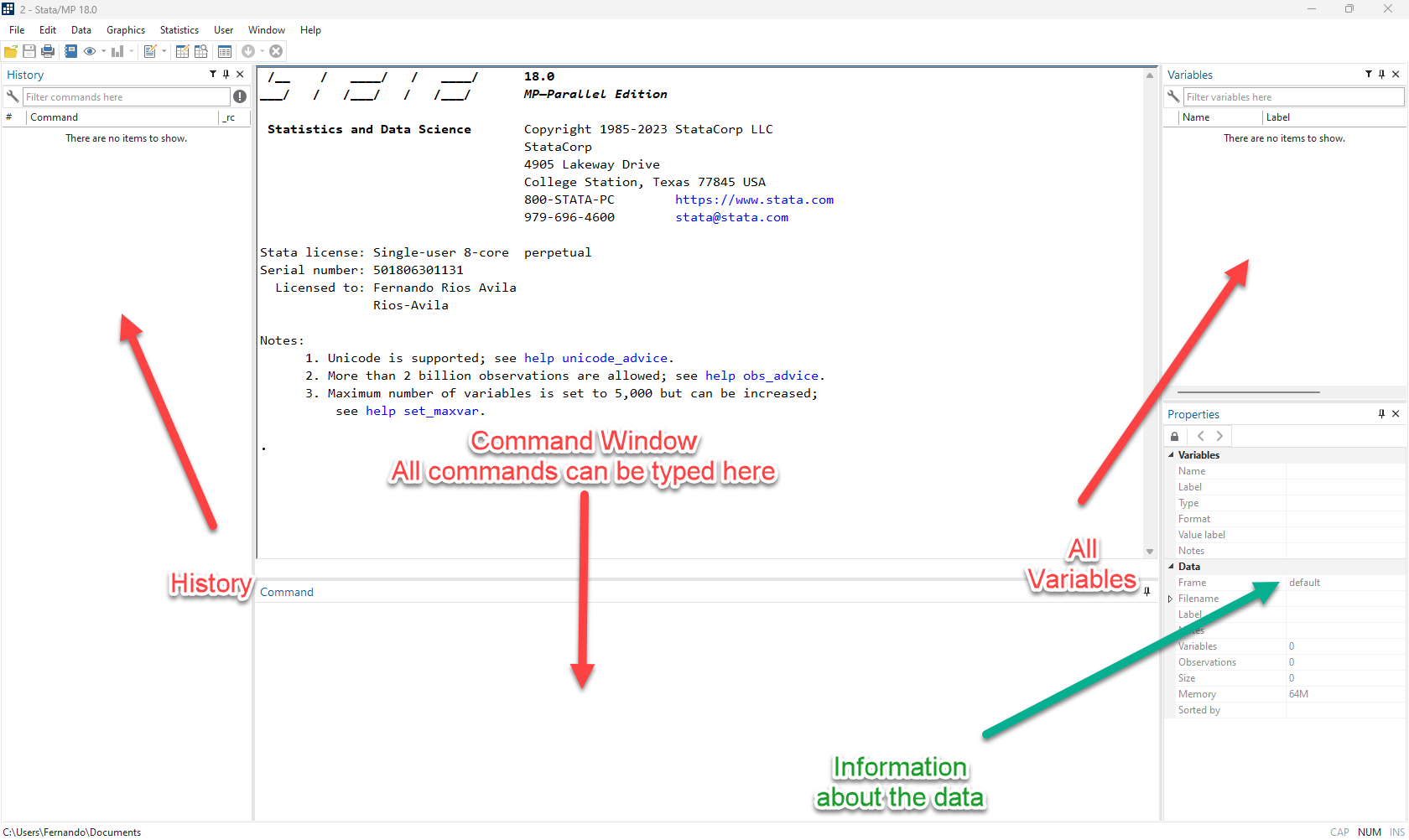
Command Window
- You can use command window to type and excute commands directly into
Stata. - Great for interactive exploration and analysis…
- But highly recommended that Final analysis is “always” done in a “do-file”
Help
- 99% of Stata commands come with Extensive help.
- If you do not know how to use a command, or about a test just “ask for help”
help help[R] help -- Display help in Stata
-------------------------------------------------------------------------------
Stata's help system
There are several kinds of help available to the Stata user. For more
information, see Advice on getting help. The information below is
technical details about Stata's help command.
-------------------------------------------------------------------------------
Syntax
help [command_or_topic_name] [, nonew name(viewername)
marker(markername)]
Menu
Help > Stata command...
Description
The help command displays help information about the specified command or
topic. help launches a new Viewer to display help for the specified
command or topic or displays help on the console in Stata for
Unix(console). If help is not followed by a command or a topic name,
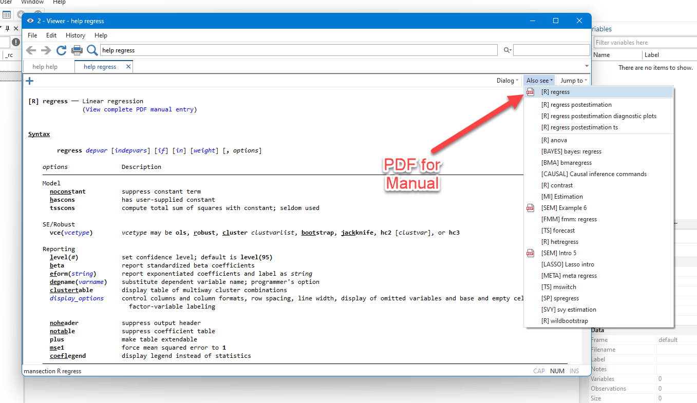
Stata displays advice for using the help system and documentation.For estimation commands, and specialized tests, help even provides links to the manuals.
The manuals have extensive detailed information on methods, formulas, references, and examples.

Of course there is 1% that is “documented/undocumented” or truly undocumented.
Most Community-contributed commands also have helpfiles, but are not always fully documented.
You could also ask for helps on “topics”:
help sample selection
Installing Programs
Stata, for all practical purposes, is self-contained.- You do not need outside sources to analyze your data, estimate models, create tables, etc.
- However, many users provide add-ons that may help to make your work “easier”
- Main Stata repository : Boston College Statistical Software Components (SSC) archive
** For using Wooldridge Book Datasets
ssc install frause, replace
** For Easiy tables
net install estout, replace from(https://raw.githubusercontent.com/benjann/estout/master/)
** My own installer for extra utilities
net install fra, replace from(https://friosavila.github.io/stpackages)
fra install fra_tools, replace- If at any point there is code that produces an error, and there is no
help, let me know.
Loading Data
StataFiles have format dta.- Loading Stata-data into
Statais very easy.- Double-click (opens a new
Stata) - Drag and Drop into your
Statainstance - Load it from menu File>open
- or using a do-file or command window
- Double-click (opens a new
- Other Formats required extra work.
- Use other software to “translate” it into Stata
- Menu: File>import> many choices
Stata System-files
. ** Most Stata example files
. ** Syntax:   sysuse  [filename], [clear]
. sysuse dir
  abortion.dta    citytemp.dta    nlsw88.dta      titanic.dta
  auto.dta        citytemp4.dta   nlswide1.dta    tsline1.dta
  auto16.dta      educ99gdp.dta   oaxaca.dta      tsline2.dta
  auto2.dta       gapminder.dta   pop2000.dta     uslifeexp.dta
  autornd.dta     gnp96.dta       ri.dta          uslifeexp2.dta
  avocado.dta     lifeexp.dta     sandstone.dta   voter.dta
  bplong.dta      mortgages.dta   scorecard.dta   xtline1.dta
  bpwide.dta      mroz.dta        snow.dta        yule.dta
  cancer.dta      network1.dta    sp500.dta
  castle.dta      network1a.dta   surface.dta
  census.dta      nhefs.dta       texas.dta

.
Other
** Web data from Stata
webuse "data-file-address", clear
** From other sites
webuse set [webaddress]
webuse data-file-address, clear
webuse set
** from frause and Wooldrige
frause , dir
frause wage1, clear
** from anyadress
use "filename-adress", clear
use "https://friosavila.github.io/playingwithstata/data2/wage1.dta", clear
Basic Data description
. sysuse auto, clear
(1978 automobile data)

. des

Contains data from C:\Program Files\Stata17/ado\base/a/auto.dta
 Observations:            74                  1978 automobile data
    Variables:            12                  13 Apr 2020 17:45
                                              (_dta has notes)
-------------------------------------------------------------------------------
Variable      Storage   Display    Value
    name         type    format    label      Variable label
-------------------------------------------------------------------------------
make            str18   %-18s                 Make and model
price           int     %8.0gc                Price
mpg             int     %8.0g                 Mileage (mpg)
rep78           int     %8.0g                 Repair record 1978
headroom        float   %6.1f                 Headroom (in.)
trunk           int     %8.0g                 Trunk space (cu. ft.)
weight          int     %8.0gc                Weight (lbs.)
length          int     %8.0g                 Length (in.)
turn            int     %8.0g                 Turn circle (ft.)
displacement    int     %8.0g                 Displacement (cu. in.)
gear_ratio      float   %6.2f                 Gear ratio
foreign         byte    %8.0g      origin     Car origin
-------------------------------------------------------------------------------
Sorted by: foreign

. list in 1/3

     +------------------------------------------------------------------------+
  1. | make        | price | mpg | rep78 | headroom | trunk | weight | length |
     | AMC Concord | 4,099 |  22 |     3 |      2.5 |    11 |  2,930 |    186 |
     |------------------------------------------------------------------------|
     |     turn     |     displa~t     |     gear_r~o     |      foreign      |
     |       40     |          121     |         3.58     |     Domestic      |
     +------------------------------------------------------------------------+

     +------------------------------------------------------------------------+
  2. | make        | price | mpg | rep78 | headroom | trunk | weight | length |
     | AMC Pacer   | 4,749 |  17 |     3 |      3.0 |    11 |  3,350 |    173 |
     |------------------------------------------------------------------------|
     |     turn     |     displa~t     |     gear_r~o     |      foreign      |
     |       40     |          258     |         2.53     |     Domestic      |
     +------------------------------------------------------------------------+

     +------------------------------------------------------------------------+
  3. | make        | price | mpg | rep78 | headroom | trunk | weight | length |
     | AMC Spirit  | 3,799 |  22 |     . |      3.0 |    12 |  2,640 |    168 |
     |------------------------------------------------------------------------|
     |     turn     |     displa~t     |     gear_r~o     |      foreign      |
     |       35     |          121     |         3.08     |     Domestic      |
     +------------------------------------------------------------------------+

.
. webuse smoking, clear
(Smoking and mortality data)

. des

Contains data from https://www.stata-press.com/data/r17/smoking.dta
 Observations:        17,260                  Smoking and mortality data
    Variables:            16                  27 Dec 2020 15:21
                                              (_dta has notes)
-------------------------------------------------------------------------------
Variable      Storage   Display    Value
    name         type    format    label      Variable label
-------------------------------------------------------------------------------
serno           int     %10.0g                Serial number
cigs            byte    %10.0g                Daily cigarette consumption
sysbp           int     %10.0g                Systolic blood pressure (mm Hg)
diasbp          float   %10.0g                Diastolic blood pressure (mm Hg)
map             float   %9.0g                 Mean arterial pressure (mm Hg)
age             byte    %10.0g                Age (years)
ht              double  %10.0g                Height (cm)
wt              double  %10.0g                Weight (kg)
chol            double  %10.0g                Cholesterol (mmol/l)
gradd1          byte    %8.0g                 Job grade 1
gradd2          byte    %8.0g                 Job grade 2
gradd3          byte    %8.0g                 Job grade 3
all10           byte    %8.0g                 Ten year mortality
pyar            double  %10.0g                Years of follow-up
chd             byte    %10.0g                Censoring (0 = censored, 1 = died
                                                of CHD)
jobgrade        byte    %10.0g                Job grade
-------------------------------------------------------------------------------
Sorted by:

. list cigs map age ht gradd1 in 1/3

     +-----------------------------------------+
     | cigs        map   age       ht   gradd1 |
     |-----------------------------------------|
  1. |    0         97    46   154.94        0 |
  2. |    0   97.66666    55   179.07        1 |
  3. |    0         82    43   173.99        1 |
     +-----------------------------------------+

.
. frause smoking, clear
(A.C.Cameron & P.K.Trivedi (2022): Microeconometrics Using Stata, 2e)

. des

Contains data from https://friosavila.github.io/playingwithstata/data2/smoking.
> dta
 Observations:         1,209                  A.C.Cameron & P.K.Trivedi
                                                (2022): Microeconometrics Using
                                                Stata, 2e
    Variables:             7                  5 Oct 2022 13:08
-------------------------------------------------------------------------------
Variable      Storage   Display    Value
    name         type    format    label      Variable label
-------------------------------------------------------------------------------
state           byte    %14.0g     state      State no
year            int     %9.0g                 Year
cigsale         float   %9.0g                 Cigarette sale per capita (in
                                                packs)
lnincome        float   %9.0g                 Log state per capita GDP
beer            float   %9.0g                 Beer consumption per capita
age15to24       float   %9.0g                 Percent of state population aged
                                                15–24 years
retprice        float   %9.0g                 Retail price of cigarettes
-------------------------------------------------------------------------------
Sorted by: year

. list in 1/3

     +-----------------------------------------------------------------------+
     |        state   year   cigsale   lnincome   beer   age15~24   retprice |
     |-----------------------------------------------------------------------|
  1. | Rhode Island   1970     123.9          .      .   .1831579       39.3 |
  2. |    Tennessee   1970      99.8          .      .   .1780438       39.9 |
  3. |      Indiana   1970     134.6          .      .   .1765159       30.6 |
     +-----------------------------------------------------------------------+

.
Summary Statistics
- Summary Statistics are essential before starting basic analysis.
Statagives you many options. Although not all of them are easy to export.
. frause oaxaca, clear
(Excerpt from the Swiss Labor Market Survey 1998)

. *summarize [varlist] [if] [in] [weight] [, options]
. summarize if female==1, sep(0)

    Variable |        Obs        Mean    Std. dev.       Min        Max
-------------+---------------------------------------------------------
      lnwage |        683    3.266761    .5700236    .507681   5.259097
        educ |        888    11.06025     2.26024          5       17.5
       exper |        683    12.13769     8.32663          0   41.91667
      tenure |        683    6.605051    6.727475          0   40.08333
        isco |        683    3.920937    1.762983          1          9
      female |        888           1           0          1          1
         lfp |        888    .7691441    .4216179          0          1
         age |        888    39.88401    10.72665         18         62
       agesq |        888    1705.666    879.4667        324       3844
      single |        888    .3018018    .4592984          0          1
     married |        888    .5236486    .4997219          0          1
    divorced |        888    .1745495    .3797953          0          1
       kids6 |        888     .286036    .6726639          0          4
     kids714 |        888        .375    .7538888          0          4
          wt |        888    .9883364    .4030975   .5302977   3.181786

.
. *   tabstat varlist [if] [in] [weight] [, options]
. tabstat educ exper tenure age married, by(female)

Summary statistics: Mean
Group variable: female (sex of respondent (1=female))

  female |      educ     exper    tenure       age   married
---------+--------------------------------------------------
       0 |   11.8004  14.07684  9.003107  38.51647  .5230567
       1 |  11.06025  12.13769  6.605051  39.88401  .5236486
---------+--------------------------------------------------
   Total |  11.40134  13.15324  7.860937  39.25379  .5233758
------------------------------------------------------------

. tabstat educ exper tenure , by(female) stats(p10 p50 p90)

Summary statistics: p10, p50, p90
Group variable: female (sex of respondent (1=female))

  female |      educ     exper    tenure
---------+------------------------------
       0 |      10.5  1.416667  .4166667
         |      10.5  11.08333      6.25
         |      17.5  31.33333     23.25
---------+------------------------------
       1 |         9      2.25  .3333333
         |      10.5     10.75      4.25
         |      12.5    23.375     15.75
---------+------------------------------
   Total |         9  1.833333  .4166667
         |      10.5  10.91667  5.291667
         |        15  28.08333  19.41667
----------------------------------------

.
. ssc install table1
checking table1 consistency and verifying not already installed...
all files already exist and are up to date.

. * see help table1
. table1, by(female) vars(lnwage contn %3.2f \ age contn %2.1f \ married bin)
  +--------------------------------------------------------------------+
  | Factor                         female = 0    female = 1    p-value |
  |--------------------------------------------------------------------|
  | N                              759           888                   |
  |--------------------------------------------------------------------|
  | log hourly wages, mean (SD)    3.44 (0.48)   3.27 (0.57)    <0.001 |
  |--------------------------------------------------------------------|
  | age of respondent, mean (SD)   38.5 (11.3)   39.9 (10.7)     0.012 |
  |--------------------------------------------------------------------|
  | married                        397 (52.3%)   465 (52.4%)      0.98 |
  +--------------------------------------------------------------------+

. qui:table1, by(female) vars(lnwage contn %3.2f \ age contn %2.1f \ married bi
> n) saving(m1.xls)
file m1.xls already exists
r(602);
You can see the file here
There are other options from
Stataas well. seehelp dtableandhelp table.Or you could construct some yourself with the help of
estoutandesttab.See here for a quick guide on tables.
Creating variables
- Two main commands:
generate(orgenfor short): Creates new variables as a function of others in the data. One can apply system functions. Example:gen var1 = 1gen var2 = _ngen wage = exp(lnwage)gen age_educ = age * educ
replace: replaces values in an already existing variable.replace wage = 0 if wage==.replace age_educ = . if female==1
egen: Advanced variable generating function. It applies a single function to a variable or list of variables to create a third one.egen wage_mean=mean(exp(lnwage)), by(female)egen wage_p10=pctile(lnwage), by(female) p(10)
- To delete a variable, you can use
drop varname/varlistordrop2 varname/varlistdropis the official. Stops if the variable does not exist.drop2an addon. Will still work even if a variable name does not exist.
Requires using full variable name.
. gen var1 = exp(lnwage)
(213 missing values generated)

. gen xar2 = exp(lnwage)+married
(213 missing values generated)

. drop x

. des var1 xar2
variable xar2 not found
r(111);
. gen xar2 = exp(lnwage)+married
(213 missing values generated)

. drop2 x
variable x not found

.
Variables Management
Statais case sensitive.- You can create variables with names
one,One,OnE,ONE, etc. - “file addresses” and commands are also case sensitive
- You can create variables with names
- In
Stata, variable names cannot can only start with a letter or “_“. Otherwise, it will give you an error. - Once variables are created, you could “label” them
label var variable_name "Description" - You can name other components of a dataset as well. See
help label
Plots in Stata
Statacan create figures and plots for data exploration
Scatter plot
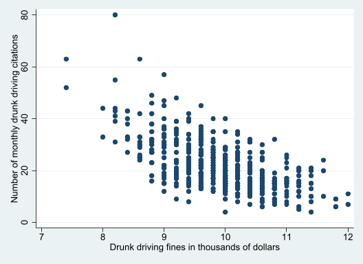
. webuse dui, clear
(Fictional data on monthly drunk driving citations)

. scatter citations fines

. 
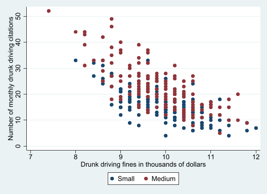
. two (scatter citations fines if csize==1)  ///
>     (scatter citations fines if csize==2), ///
>     legend(order(1 "Small" 2 "Medium"))

. 
- The limitation. User written plotting commands do not interact well with Official plotting commands.
Saving your work
Command Window is effective to provide interactive analysis
At the end of your session, you can recover everything you did, clicking on the History Section, and save everythig, or just specific commands.
The best approach, however, is to ALWAYS use a do-file.
First of all: Create a working directory. A folder in your computer that will hold your project, work, paper, homework, etc. (highly recommended)
Create a dofile: For simple projects a single file will suffice, but multiple may be needed for larger ones.
To start a dofile, simply type
doedit "filename"in your command window.- If file exists in your “working directory” (type
cdto see where you “are”), it will open it. - Otherwise, a new file will be created
- If file exists in your “working directory” (type
do-filesare the best approach to save your work, and keep track of your analysis.General Suggestion: Allways add comments to it, to know what you are doing
*  You can always Start a command like this
// Or like this
/*
But you can always add a large comment using "/*" to start
and "*/" to end it
*/

/* You could also add comments at the end of a command */
sysuse auto, clear  // Loading Auto Dataset, after "clearing" the one currently in memory

// Or as I did before, break a long command in various lines using "///"
// Comments after "///" are possible
regress price     /// Dep variable
        mpg       /// indep variable
        i.foreign, /// Foreign Dummy
        robust     // Request Robust Standard errors.

** Last one has only two "/", because line ends there
(1978 automobile data)
Linear regression Number of obs = 74
F(2, 71) = 12.72
Prob > F = 0.0000
R-squared = 0.2838
Root MSE = 2530.9
------------------------------------------------------------------------------
| Robust
price | Coefficient std. err. t P>|t| [95% conf. interval]
-------------+----------------------------------------------------------------
mpg | -294.1955 60.33645 -4.88 0.000 -414.503 -173.8881
|
foreign |
Foreign | 1767.292 607.7385 2.91 0.005 555.4961 2979.088
_cons | 11905.42 1362.547 8.74 0.000 9188.573 14622.26
------------------------------------------------------------------------------Estimation Commands
- Most commands in
Statahave the following syntax:
[by varlist:/prefix] command [varlist] [if exp] [in range] [weight] [using filename] [,options]- everything in
[]are optional. [by varlist:/prefix]:byis used to execute the command by groups.
prefixto request additional manipulation (advanced use)command: The command itself that will process the datavarlist: For Estimation commands include the dependent (first) and independent variables (everything else)[if exp] [in range]: To restrict samples[weight]: Request the use of weights ie:[fw = wgt_var]or[pw = wgt_var][using filename]: Some commands allow you to use this to work with not-yet loaded datasets or files.[options]: Options requesting specific behaivior, statistics, etc
Adv options for saving work.
- Use
github, as an additional data-repository - Combine
Stata,pythonandnbstatto createJupyter notebooks. - You can also use Quarto to create full dynamic reports.