Probability and Classification

Am I a man, or am I a muppet?

Fernando Rios-Avila

Levy Economics Institute

November 20, 2024

Motivation

• Say you work for a consultancy agency helping a bank. You are asked to predict which firms will default on their loans.
  • What would be better: a model that predicts probabilities or a model that classifies firms into default or not default?
  • How do you use to decide which firms should get a loan.
• Companies need to assess the likelihood of their suppliers or clients staying in business, as it impacts their own operations.
  • How to use historical data on company exits, along with key features, to predict the probability of a company’s exit.

Previously on DA

• In the previous weeks, we have covered the basics of prediction when the target is quantitative.
  • Almost stright forward: predict the value of the target. Consider many specifications and pick the best one.
• We also cover the basic of probability modeling
  • LPM, Logit and probit models: When your dependent variable is Binary.
• However, we have not fully cover how to use these models for prediction.

Prediction with qualitative target

• Consider cases where \(Y\) is qualitative
  • Whether a debtor defaults (will default) on their loan
  • Email is spam or not
  • Game result is win / lose (no draw).
• For all this cases, the target (dep variable) is binary.
• The question is: Given this, What is the best way to predict the target?
  • Predict the probability of “success” (default, spam, win)
  • or make a classification (default, spam, win) based on a probability.

Classification: The extra step

The process

• Predict probability: We have done this.
  • Predicted probability between 0 and 1 (logit, probit or LPM in extreme cases)
  • For each observation we predicted a probability. Often that is it.

if logit: \[\Pr[y_i = 1|x_i] = \Lambda \times (\beta_0 + \beta_1x_i) = \frac{\exp (\beta_0 + \beta_1x_i)}{1 + \exp (\beta_0 + \beta_1x_i)}\]

• Thats it! You can probably go couple of steps further and use various specifications, as well as LASSO (for logit) to pick the best model.

• Best model can still be picked based on RMSE, brier score or Calibration.

Refresher: Probability Models

• LPM - not this time: Predicted value MUST be between 0 and 1

• Logit or probit (or other non-linear probability models)

• Nonlinear probability models \[\Pr[y_i = 1|x_i] = \Lambda(\beta_0 + \beta_1x_i) = \frac{\exp (\beta_0 + \beta_1x_i)}{1 + \exp (\beta_0 + \beta_1x_i)}\]

  • Predicted probability between 0 and 1
  • Starts with a linear combination of the explanatory variables
  • Multiplies them with coefficients, just like linear regression
  • And then transforms that into something that is always between 0 and 1, the predicted probability.

What’s New with Binary target?

• The predicted Probability is not a value.
• Desire to classify
  • assign 0 or 1
  • based on a probability that comes from a model
  • But how?
• We also need new measures of fit
  • Some based on probabilities
  • Others based on classification

What’s NOT new with Binary target?

• Need best fit
  • With highest external validity
• Usual worries: overfit
  • Cross-validation helps avoid worst overfit
• Models similar to those used earlier
  • Regression-like models (probability models)
  • Tree-based models (CART, Random Forest) <- We will not cover this

Probability prediction and process

• We build models to predict probability when:
  • aim is to predict probabilities – (Duh!)
  • aim is to classify (predict 0 or 1) – (we need probabilities first)
• Build models
  • several Logit models by domain knowledge
  • LASSO - Logit LASSO
• Pick the best model via cross-validation using RMSE / Brier score
  • Or other LOSS function, if you have one

Classification process

• After you predict your conditional probability, you can make classifications based on some threshold or Rule.
  • For example if \(\Pr[y = 1] > 0.5\) then predict 1, otherwise predict 0
  • But we can choose any threshold. but how? (say top 10%?)
• We need to consider that we can make errors
  • False negative
  • False positive
• Thus we need to consider a threshold that minimizes the expected errors

Classification Table: Confusion Matrix

	\(y_j = 0\)	\(y_j = 1\)	Total
\(\hat{y}_j = 0\)	TN	FN	TN + FN
Predicted negative	(true negative)	(false negative)	(all classified negative)
\(\hat{y}_j = 1\)	FP	TP	FP + TP
Predicted positive	(false positive)	(true positive)	(all classified positive)
Total	TN + FP	FN + TP	TN + FN + FP + TP
(all actual negative)	(all actual positive)	(N, all observations)

Classification Table: making errors

	\(y_j = 0\)	\(y_j = 1\)	Total
\(\hat{y}_j = 0\)	Predict firm stay	Predict firm stay	TN + FN
Predicted negative	(Firm did stay )	(Firm exited )	(all classified stay )
\(\hat{y}_j = 1\)	Predict firm exit	Predict firm exit	FP + TP
Predicted positive	(Firm stayed )	(Firm did exit)	(all classified exit)
Total	TN + FP	FN + TP	TN + FN + FP + TP
(all actual stay )	(all actual exit)	(N, all observations)

Measures of classification

There are several measures of classification, each with a different focus.

• Accuracy \(=(TP+TN)/N\)
  • The proportion of rightly guessed observations
  • Hit rate
• Sensitivity \(=TP / (TP+FN)\)
  • The proportion of true positives among all actual positives
  • Probability of predicted \(y\) is 1 conditional on \(y = 1\)
• Specificity \(= TN/(TN+FP)\)
  • The proportion of true negatives among all actual negatives
  • Probability predicted \(y\) is 0 conditional on \(y = 0\)

Theory: The ROC

Sensitivity vs Specificity

Measures of classification

• The key point is that there is a trade-off between making false positive and false negative errors.
• This is the essential insight in classification
• This can be expressed with specificity and sensitivity.
  • if your Threshold is low, You can detect all the positives, but you will also detect many false positives. Sensitivity is high.
  • if your Threshold is high, You can detect all the negatives, but you will also detect many false negatives. Specificity is high.

ROC Curve

• The ROC curve is a popular graphic for simultaneously displaying specificity and sensitivity for all possible thresholds.
• ROC: Receiver operating characteristic curve
  • Name from engineering
• For each threshold, we can compute confusion table \(\rightarrow\) calculate sensitivity and specificity
• Then, we can plot sensitivity vs 1-specificity for all thresholds
  • Horizontal axis: False positive rate (one minus specificity) = the proportion of FP among actual negatives
  • Vertical axis: is true positive rate (sensitivity) = proportion of TP among actual positives

ROC Curve Intuition

• Consider this:
  • If the threshold is 0, we predict all observations as 1. The sensitivity is 1, but the specificity is 0.
  • If the threshold is 1, we predict all observations as 0. The sensitivity is 0, but the specificity is 1.
  • The “ideal” threshold is somewhere in between.
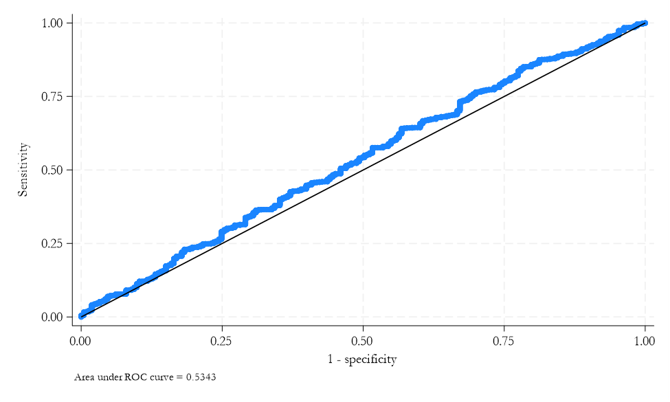
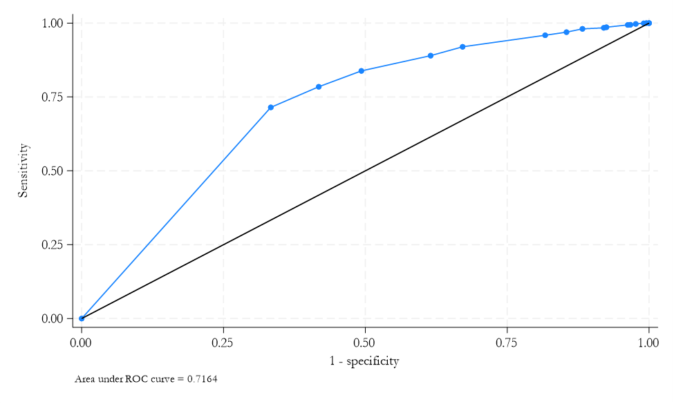
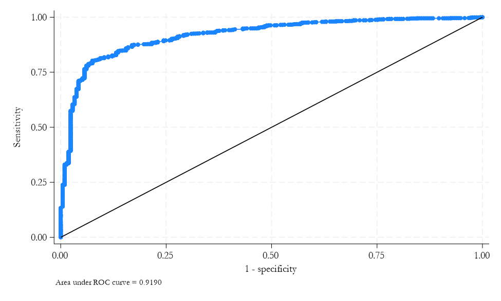
• ROC curve shows how true positives and false positives increases relative to each other.

ROC Curve Intuition

• Random Covariate
• Nof Children
• Full Model

Area Under ROC Curve

• ROC curve: the closer it is to the top left column, the better the (insample) prediction.
• Area under ROC (AUC) curve summarizes quality of probabilistic prediction
  • For all possible threshold choices
  • Area \(=\) 0.5 if random classification
  • Area \(>\) 0.5 if curve mostly over 45 degree line
• AUC is a good statistic to compare models
  • Defined from a non-threshold dependent model (ROC)
  • The larger the better
  • Ranges between 0 and 1.

Stata Corner

• Logit estimation: logit y x1 x2 x3
• Predict probabilities: predict yhat, pr
• Classification:
  • gen yhat_class = (yhat > 0.5)
  • estat classification
• ROC curve: lroc

Model selection Nr.1: Probability models

• Model selection when we have no loss function, based on probability models only
  • Predict probabilities (No actual classification)
  • Use predicted probability to calculate RMSE
  • Pick by smallest RMSE
• Or
  • Draw up ROC curve and get AUC, Pick the model with the largest AUC
  • More frequently used in practice
  • Less sensitive to class imbalance
• In practice, AUC is more frequently used

Theory: Classification and loss function

How we make classification from predicted probability?

• We set a threshold!
• The process of classification
  • If probability of event is higher than this threshold\(\rightarrow\) assign (predict) class 1; and 0 otherwise.
• Who sets the threshold?
  • Usually approximated by 0.5
  • or by the frequency of the event in the data

Classification: select the threshold with loss function

• Find optimal threshold with loss function.
  • A loss function is a dollar value assigned to false positive and false negative.
  • Most often the costs of FP and FN are very different.

Consider loss function

\[E[loss] = \Pr[FN] \times loss(FN) + \Pr[FP] \times loss(FP)\]

• In ideal case, the minimization of this suggests that optimal threshold is:

\[\text{Threshold} = \frac{loss(FP)}{loss(FN) + loss(FP)}\]

• Or we can try finding the threshold that minimizes the expected loss using Cross-validation. (Software issue)

When to use Formula

• Formula
  • When dataset is “large”
  • When our model has a “good” fit \(\text{Threshold}_{\min E (loss)} = \frac{loss(FP)}{loss(FN) + loss(FP)}\)
• In practice
  • Pro: easy to use, often close enough
  • Con: not the best cutoff, especially for smaller data, and poorer model

Class imbalance

• A potential issue for some dataset - relative frequency of the classes.
• Class imbalance = the event we care about is very rare or very frequent (\(\Pr(y = 1)\) or \(\Pr(y = 0)\) is very small)
  • Fraud, Sport injury
• What is rare?
  • Something like 1%, 0.1%. (10% should be okay.)
  • Depends on size: in larger dataset we can identify rare patterns better.
• Consequence: Hard to find those rare events.
  • You may be able to identify some patterns by chance.

Class imbalance: the consequences

• Methods we use are not good at handling it.
  • Both for the models to predict probabilities, and for the measures of fit used for model selection.
• The functional form assumptions behind the logit model tend to matter more, the closer the probabilities are to zero or one.
• Cross-validation can be less effective at avoiding overfitting with very rare or very frequent events if the dataset is not very big. (Many samples will not even have the event.)
• Usual measures of fit can be less good at differentiating models.
• Consequence: Model fitting and selection setup not ideal

Class imbalance: what to do

• What to do? Two key insights.
  1. Know when it’s happening, and be ready for poor performance.
  2. May need an action: rebalance sample to help build better models
• Downsampling – randomly drop observations from frequent class to balance out more
  • Before: 100,000 observations 1% event rate (99,000 \(y = 1\), 1,000 \(y = 0\))
  • After 10,000 observations 10% event rate (9,000 \(y = 1\), 1,000 \(y = 0\))
• Over-sampling of rare events
• try Smart algorithms: Synthetic Minority Over-Sampling Technique (SMOTE)
  • Create synthetic observations that are similar to the rare events
  • synthetic rare = Combination of rare and infrequent events

Case study

Firm exit case study: Case study: background

• Banks and business partners are often interested in the stability of their customers.
• Predicting which firms will be around to do business with is an important part of many prediction projects.
• Working with financial and non-financial information, your task may be to predict which firms are more likely to default than others.
• Goal: Predict corporate default - exit from the market.
  • We have to figure out and decide on target, features, etc.

Firm exit case study: bisnode-firms dataset

• Firm data
• Many different type of variables
  • Financial, Management, Ownership, Status (HQ)
• Dataset is a panel data
• Rows are identified by company id (comp-id) and year.
• We’ll focus on a cross-section of 2012.

Firm exit case study: Label (target) engineering

• Defining our target. There is no “exit” - we have to define it!
• Option: If a firm is operational in year \(t\), but is not in business in \(t + 2\) -> Exit.
• This definition is broad
  • Defaults / forced exit
  • Orderly closure
  • Acquisitions

Firm exit case study: Sample design

• Look at a cross section in 2012
  • If alive in Year=2014, status_alive=1
• Keep if established in 2012
• We do not care about all firms. Not very small and very large
  • Below 10 million euros
  • Above 1000 euros
• Hardest call: keep when important variables are not missing
  • Balance sheet like liquid assets
  • Ownership like foreign
  • Industry classification
• End with 19K observation, 20% default rate

Firm exit case study: Features - overview

• Key predictors
  • size: sales, sales growth
  • management: foreign, female, young, number of managers
  • region, industry, firm age
  • other financial variables from the balance sheet and P&L.
• For financial variables, we use ratios (to sales or size of balance sheet).
• Here it will turn out be important to look at functional form carefully, especially regarding financial variables.
• Mix domain knowledge and statistics.
• Plenty of analyst calls.

Firm exit case study: Feature engineering

• Growth rates
  • 1 year growth rate of sales. Log difference.
  • Could use longer time period, but Lose observations
    
• Ownership, management info
  • Keep if well covered, impute some, but drop if key vars missing
  • Sometimes simplify (unless big data): ceo_young = ceo_age_mod <40 & ceo_age_mod >15
• Industry categories - need simplify
• Foreign ownership - above a threshold
• Numerical variables from balance sheet: Check functional form - logs, polynomials

Firm exit case study: Feature engineering tools

• Check coverage (missing values)
• Decide on imputation vs drop
• Categorical (factor) variables
• Numerical variables
  • Check functional form - logs, polynomials
  • Look at relationships in scatterplot, loess and decide

Firm exit case study: Feature engineering

• May need to make cleaning steps.
• Create binary variables (flags) when implementing changes to values.
• When financial values are negative: replace with zero and add a flag to capture imputation.
  • Zeros will not work with logs.
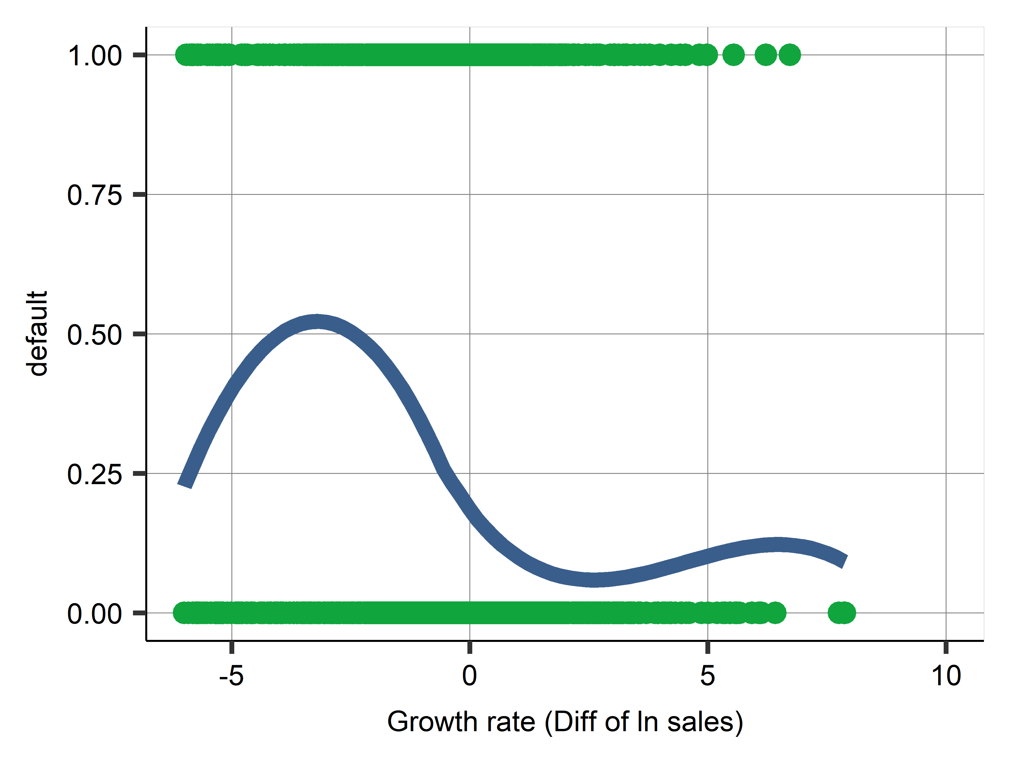
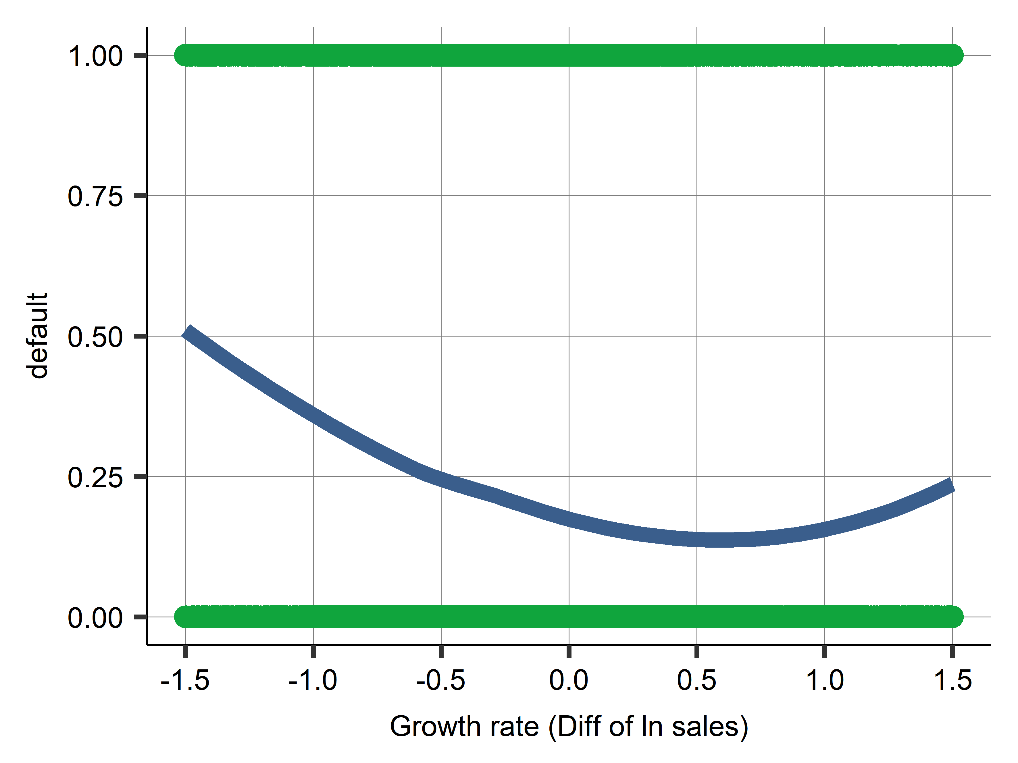
• Annual growth in sales (difference in log sales) vs default
  • Try editing variables by Winsorizing and adding flags for extreme values.
  • Some ODD shapes due to extreme values.

The Weird Shape

Winzordize

Firm exit case study: Winsorizing

• When edge of a distribution is weird…
• Winsorizing is a process to keep observations with extreme values in sample
  • for each variable, we
    • identify a threshold value, and replace values outside that threshold with the threshold value itself
    • and add a flag variable.
• Two ways to do it:
  • an automatic approach, where the lowest and highest 1 percent or 5 percent is replaced and flagged.
  • Pick thresholds by domain knowledge as well as by looking at lowess. Preferred.

Firm exit case study: Firm sales growth

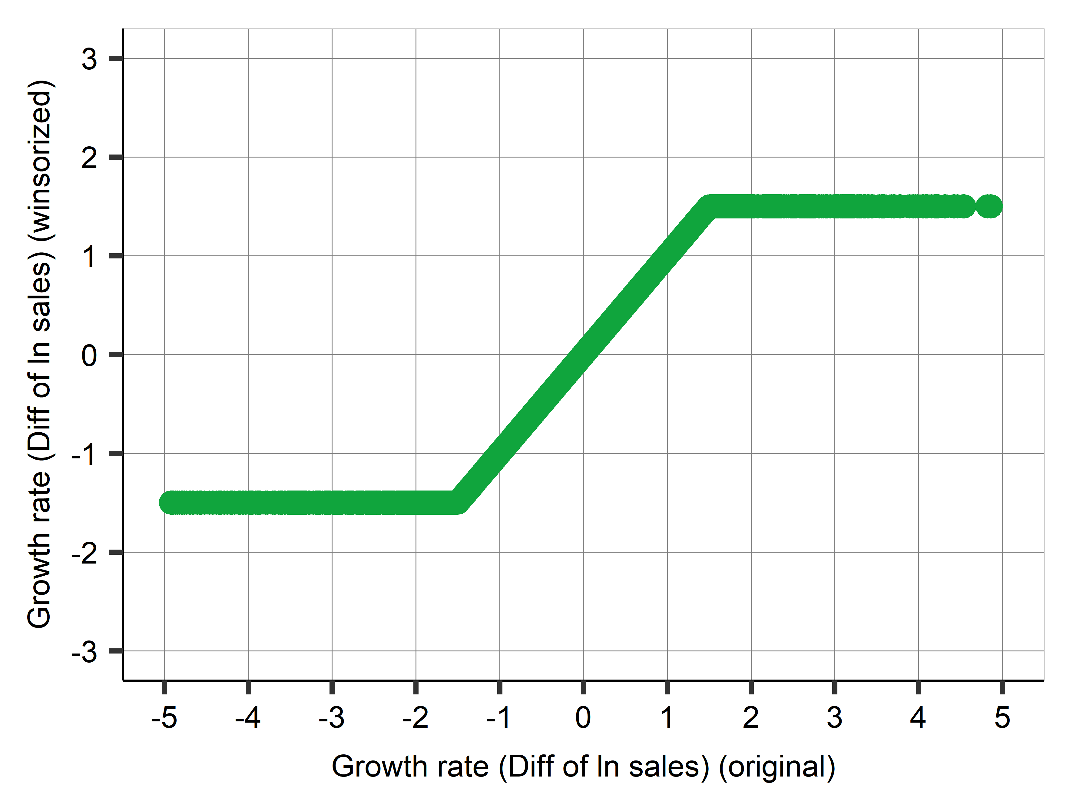
• The winsorized value simply equals original value in a range and flat below/after.

Firm exit case study: Model features 1

• Firm: Age of firm, squared age, a dummy if newly established, industry categories, location regions for its headquarters, and dummy if located in a big city.
• Financial 1: Winsorized financial variables: fixed, liquid (incl current), intangible assets, current liabilities, inventories, equity shares, subscribed capital, sales revenues, income before tax, extra income, material, personal and extra expenditure.
• Financial 2: Flags (extreme, low, high, zero - when applicable) and polynomials: Quadratic terms are created for profit and loss, extra profit and loss, income before tax, and share equity.
• Growth: Sales growth is captured by a winsorized growth variable, its quadratic term and flags for extreme low and high values.

Firm exit case study: Model features 2

• HR: For the CEO: female dummy, winsorized age and flags, flag for missing information, foreign management dummy; and labor cost, and flag for missing labor cost information.
• Data Quality: Variables related to the data quality of the financial information flag for a problem, and the length of the year that the balance sheet covers.
• Interactions: Interactions with sales growth, firm size, and industry.

Firm exit case study: Models

Models (number of predictors)

• Logit M1: handpicked few variables (\(p = 11\))
• Logit M2: handpicked few variables + Firm (\(p = 18\))
• Logit M3: Firm, Financial 1, Growth (\(p = 35\))
• Logit M4: M3 + Financial 2 + HR + Data Quality (\(p = 79\))
• Logit M5: M4 + interactions (\(p = 153\))
• Logit LASSO: M5 + LASSO (\(p = 142\))
• Number of coefficients = N of predictors +1 (constant)

Firm exit case study: Data

• \(N = 19,036\)
• \(N = 15,229\) in work set (80%)
• Cross validation 5x training + test sets
  • Used for cross-validation
• \(N = 3,807\) in holdout set (20%)
  • Used only for diagnostics of selected model.

Firm exit case study: Comparing model fit

	Variables	Coefficients	CV RMSE
Logit M1	4	12	0.374
Logit M2	9	19	0.366
Logit M3	22	36	0.364
Logit M4	30	80	0.362
Logit M5	30	154	0.363
Logit LASSO	30	143	0.362

• 5-fold cross-validated on work set, average RMSE
• Will use Logit M4 model as benchmark

Classification

• Picked a model on RMSE/Brier score
• For classification, we will need a threshold

Firm exit case study: ROC curve

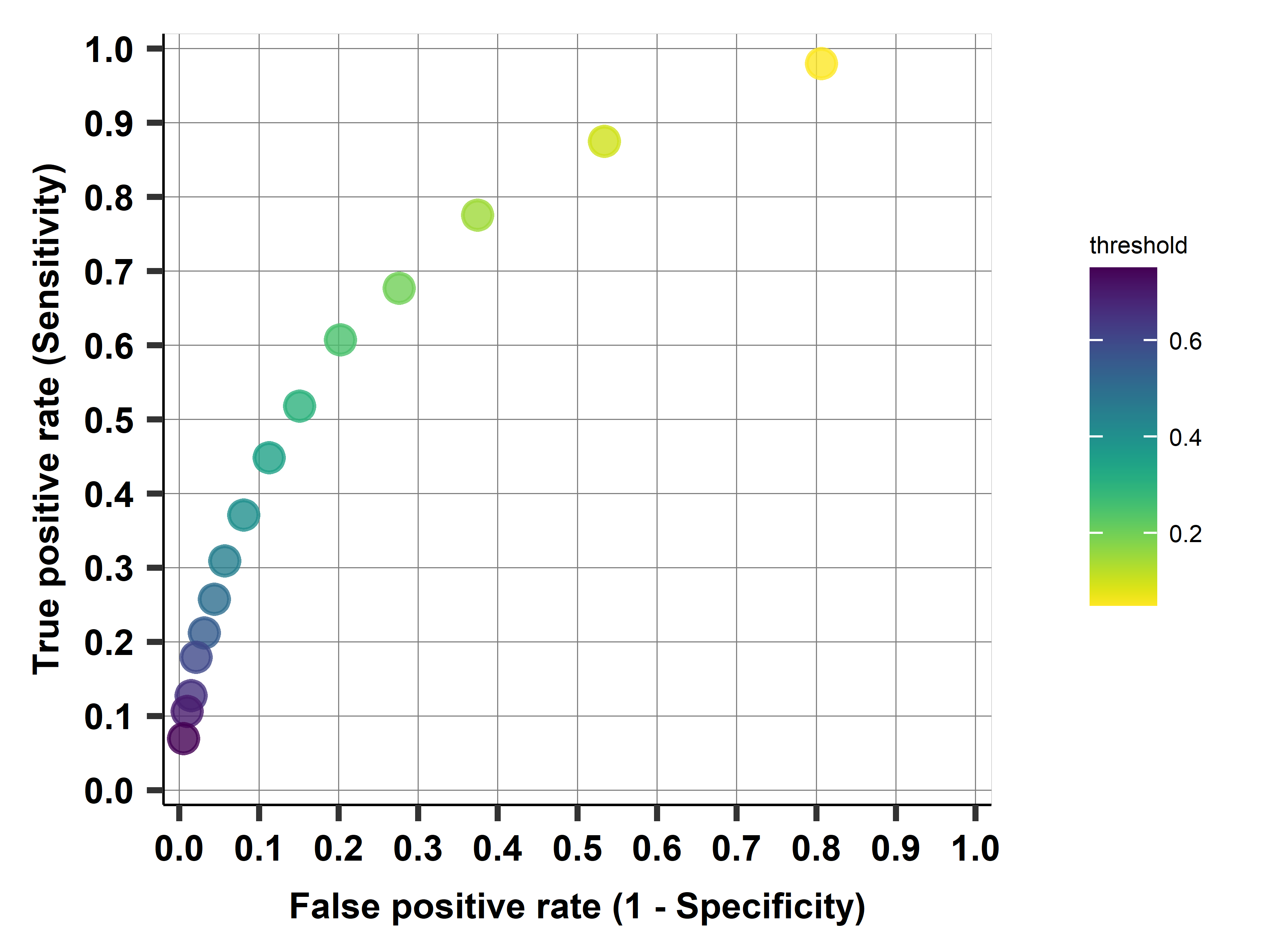
• ROC curve shows trade-off for various values of the threshold
• Go through values of the ROC curve for selected threshold values, between 0.05 and 0.75, by steps of 0.05

Firm exit case study: AUC

Model	RMSE	AUC
Logit M1	0.374	0.738
Logit M2	0.366	0.771
Logit M3	0.364	0.777
Logit M4	0.362	0.782
Logit M5	0.363	0.777
Logit LASSO	0.362	0.768

• Can calculate the AUC for all our models
• Model selection by RMSE or AUC
• Here: same (could be different if close)

Firm exit case study: Comparing two thresholds

• Take the Logit M4 model, predict probabilities and use that to classify on the holdout set
• Two thresholds: 50% and 20%
• Predict exit if probability > threshold

Firm exit case study: Comparing two thresholds

	Threshold: 0.5			Threshold: 0.2
	Actual stay	Actual exit	Total	Actual stay	Actual exit	Total
Predicted stay	75%	15%	90%	57%	7%	64%
Predicted exit	4%	6%	10%	22%	14%	36%
Total	79%	21%	100%	79%	21%	100%

Firm exit case study: Threshold choice consequences

• Having a higher threshold leads to
  • fewer predicted exits:
    • 10% when the threshold is 50% (36% for threshold 20%).
  • fewer false positives (4% versus 22%)
  • more false negatives (15% versus 7%).
• The 50% threshold leads to a higher accuracy rate than the 20% threshold
  • 50% threshold: 75% + 6% = 81%
  • 20% threshold: 57% + 14% = 71%
  • even though the 20% threshold is very close to the actual proportion of exiting firms.

Summary

First option: no loss fn

• On the work set, do 5 fold CV and loop over models
• Do Probability predictions
• Calculate average RMSE on test for each fold
• Draw ROC Curve and calculate AUC for each fold
• Pick best model based on avg RMSE
• Take best model and estimate RMSE on holdout\(\rightarrow\)best guess for live data performance
• Output: probability ranking - most likely to least likely.
• Show ROC curve and confusion table with logit on holdout 4 at \(t = 0.5\) and \(t = 0.2\) - to illustrate trade-off.

Firm exit case study: The loss function

• Loss function = FN, FP
• What matters is FN/FP
• FN=10
  • If the model predicts staying in business and the firm exits the market (a false negative), the bank loses all 10 thousand euros.
• FP=1
  • If predict exit and the bank denies the loan but the firm stays in business in fact (a false positive), the bank loses the profit opportunity of 1 thousand euros.
• With correct decisions, there is no loss.

Firm exit case study: Finding the threshold

• Find threshold by formula or algo
• Formula: the optimal classification threshold is \(1/11 = 0.091\)
• Algo: search thru possible cutoffs

Firm exit case study: Finding the threshold

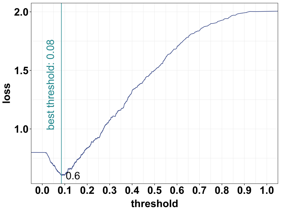
• Consider all thresholds \(T = 0.01, 0.02—1\)
• Calculate the expected loss for all thresholds
• Pick when loss function has the minimum
• Done in CV, this is fold Nr.5.

Firm exit case study

• Model selection process
  • Predict probabilities
  • Use predicted probabilities and loss function to pick optimal threshold
  • Use that threshold to calculate expected loss
  • Pick model with smallest expected loss (in 5-fold CV)
• We run the threshold selection algorithm on the work set, with 5-fold cross-validation.
• Best is model Logit M4
• the optimal classification threshold by algo is 0.082. Close to formula (0.091)
• The average expected loss of 0.64.

Firm exit case study:Summary of process with loss function

• On the work set, do 5 fold CV and loop over models
• Do Probability predictions
• Calculate average RMSE on each test folds
• Draw ROC Curve and find optimal threshold with loss function (1,10)
  • show: threshold search - loss plots and ROC curve for fold 5
• Summarize: for each model: average of optimal thresholds, threshold for fold 5, average expected loss, expected loss for fold Nr.5.
• Pick best model based on average expected loss
• Take best model, re-estimate it on work set + find optimal threshold and estimate expected loss on holdout set

Summary

• Decide whether the goal is predicting probabilities or classification.
• The outcome of prediction with a binary target variable is always the predicted probabilities as a function of predictors.
• When our goal is probability prediction, we should find the best model that predicts probabilities by cross-validation + RMSE/AUC.
• When our goal is classification, we should find the best model that has the smallest expected loss.
  • With formula for threshold or search algorithm
  • Finding the optimal classification threshold needs a loss function.

Summary

• Without a loss function, no classification.
• If you don’t have one, make it up.
• Don’t rely on default 0.5.